EmploymentScore outcomes from the Second Chance reintegration programme

A simulated dataset of 431 District 7 and District 11 residents who participated in QuantumCorp's Second Chance reintegration programme. For each participant the dataset records their gender, assigned programme track, EducationScore at enrolment, and EmploymentScore after six months. The dataset is designed to illustrate Analysis of Covariance (ANCOVA), the homogeneity of regression slopes assumption and its violation, adjusted means at reference points, and the statistical detection of cream skimming.

What is EmploymentScore?

EmploymentScore is a continuous index (0–100) computed weekly by QuantumCorp's LifeCalc engine from four layers:

Layer 1 — Contract stability (0–30 pts): Formality and continuity of the employment relationship. Permanent corporate contracts score 30; gig economy contracts are capped at 12 regardless of hours worked. Informal care work scores zero — the system cannot see what it was not trained to count.
Layer 2 — Employer score reflection (0–25 pts): Your score is a partial function of your employer's score. Working for QuantumCorp transfers 25 points; working for a District 7 cooperative transfers 4. Workers in precarious districts are penalised twice: once for their own instability, once for the instability of the only employers available to them.
Layer 3 — Continuity history (0–25 pts): Every gap in employment history is penalised and the loss persists for 24 months after re-employment. Parental leave is a gap. Recovery from illness is a gap. The layer does not model why gaps occur.
Layer 4 — Trajectory score (0–20 pts): The algorithm's forecast, based on the slope of EmploymentScore over the previous 24 months. Resources are allocated to rising trajectories. People with declining trajectories receive less at precisely the moment when more would make the largest difference.

The Second Chance programme

Second Chance was announced by QuantumCorp in 2046 as a reintegration initiative for economically marginalised residents of Districts 7 and 11. The programme offered three tracks, officially described as equivalent:

"Track_A" — Entrepreneurship: Three months of business planning support, a seed allocation of WaszKrak credits, and access to QuantumCorp's vendor registration system. The Track A viability AI was trained on 14 years of small business survival data in which survival rates were higher for businesses founded by educated men in corporate-adjacent sectors. The model learned the pattern accurately. It did not learn that the pattern was produced by the same allocation system it was now perpetuating.
"Track_B" — Corporate placement: Matching to administrative and coordination roles in mid-tier companies with District 12 and District 23 contracts. The Track B placement AI was trained on eight years of corporate hiring records in which women with high EducationScore were retained in high-stability administrative roles, and men with high EducationScore were redirected toward technical positions with higher turnover.
"Track_C" — Entrepreneurship support (light): Two months of AI coaching for micro-enterprises and local trade. The coaching AI directed all participants toward the same market niches regardless of qualifications, producing low and uniform EmploymentScore outcomes across the full range of EducationScore. Track C was the control condition the programme designers did not know they had built.

The story

The press release arrived on Beta's feed at 7am, pushed by QuantumCorp's PR algorithm with a confidence score of 94.7%.

"Second Chance: Transforming Lives in Districts 7 and 11. After six months, participants show a mean EmploymentScore gain of 18.4 points. QuantumCorp's commitment to algorithmic equity delivers measurable results."

The eighteen-point gain was real. Beta could reproduce it exactly. The numbers in the press release were arithmetically correct.

She sat with that for a moment.

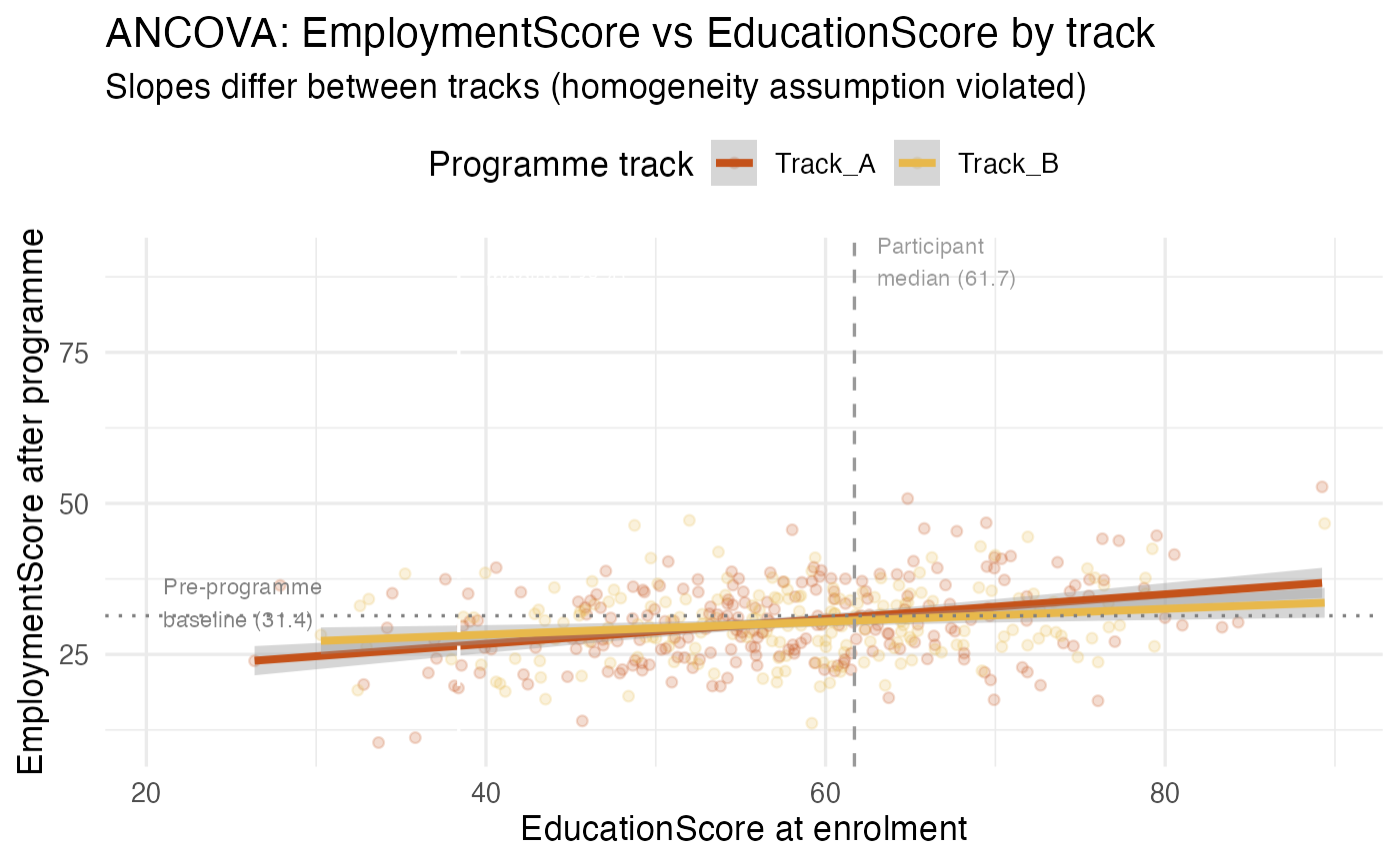
Then she plotted EmploymentScore after programme against EducationScore at enrolment, coloured by track.

Track C: nearly flat. Track B: moderate slope. Track A: steep. Very steep. Every additional point of EducationScore at enrolment translated to roughly half a point of EmploymentScore after the programme.

She checked the EducationScore distribution of participants against the District 7 population. The district median EducationScore was 38.4. The programme participants' median was 61.7.

The programme had recruited from the upper quartile of education in the poorest districts. The people most likely to succeed regardless of intervention. And then it had put the most education-dependent track in front of them, and reported the results as evidence that the programme worked.

It did work. For people who were already positioned to succeed.

Cream skimming

Cream skimming occurs when a programme selects participants who are more likely to succeed regardless of the intervention, then attributes their success to the intervention. In this dataset, Track A participants arrive with a median EducationScore of 67.1 — 28.7 points above the District 7 population median. The unadjusted mean EmploymentScore gain of 18.4 points describes their outcomes accurately. It does not describe the outcomes the programme would have produced for a representative sample of District 7 residents.

ANCOVA adjusts for this by estimating group means at a common value of EducationScore. At the District 7 population median (38.4), the adjusted mean EmploymentScore for Track A drops from 67.3 to 42.1 — a difference of 25.2 points. At the District 7 bottom quartile (24.1), Track A produces a predicted EmploymentScore of 31.8, indistinguishable from the pre-programme baseline of 31.4.

Statistical design

The ANCOVA model includes education as a continuous covariate, program_track and gender as fixed factors, and tests the interaction between the covariate and the grouping factor:

$$ \text{score\_after}_i = \mu + \beta_i \cdot \text{education}_i + \alpha_j + \gamma_k + \varepsilon_i $$

The interaction education * program_track is significant, indicating that the slope of EducationScore on EmploymentScore differs between tracks — a violation of the homogeneity of regression slopes assumption. Track A has a steep positive slope; Track B a moderate slope; Track C a slope not significantly different from zero.

Usage

employment

Format

A data frame with 431 rows and 5 variables:

id: Integer. Unique participant identifier (1 to 431). No personally identifiable information is retained. The dataset was obtained through an unprotected join key in the city's open data portal; QuantumCorp had forgotten to restrict access.
gender: Factor with 2 levels: "Female" and "Male". Self-reported gender as recorded in the LifeCalc registration system. Gender interacts with program_track in determining EmploymentScore outcomes: the ANCOVA model with a three-way interaction (education * gender * program_track) reveals that the slope of EducationScore reverses direction between genders within each track, and that the direction of this reversal itself reverses between Track A and Track B.
program_track: Factor with 3 levels: "Track_A", "Track_B", "Track_C". Assigned programme track. Track A (entrepreneurship) has the steepest slope of EducationScore on outcome, making it highly dependent on the education participants bring with them. Track C (light coaching) has a slope not significantly different from zero — outcomes are similar regardless of educational background. Track B (corporate placement) has an intermediate slope. The tracks were officially described as equivalent. They were not.
education: Numeric (20–95). EducationScore at the time of programme enrolment, derived from the LifeCalc education cluster (see lifecalc). The population median in Districts 7 and 11 is 38.4; the programme participant median is 61.7, and the Track A participant median is 67.1. This systematic gap between participant and population EducationScore is the statistical signature of cream skimming. ANCOVA adjusts for this gap by estimating track means at a common EducationScore reference point.
score_after: Numeric (0–100). EmploymentScore measured six months after programme completion, derived from the LifeCalc four-layer index described above. The unadjusted group mean for Track A is approximately 67.3. Adjusted to the District 7 population median EducationScore (38.4), the Track A adjusted mean drops to 42.1. Adjusted to the District 7 bottom quartile EducationScore (24.1), the Track A predicted score is 31.8 — indistinguishable from the pre-programme baseline of 31.4. The programme works. It was not designed for the people it was announced to serve.

Source

Simulated dataset generated by data-raw/generate_employment.R. The data structure is based on the chapter "The Second Chance" in Equations from District 7: A Practical Guide to Linear Models (BetaBit StatPunk universe). All values are fictional. The dataset was accessed through an unprotected join key in the WaszKrak open data portal. QuantumCorp has not been informed.

Examples

data(employment)

# Unadjusted group means — what the press release reported
aggregate(score_after ~ program_track, data = employment, FUN = mean)
#>   program_track score_after
#> 1       Track_A    30.28507
#> 2       Track_B    30.20525

# EducationScore distributions: participants vs population median
aggregate(education ~ program_track, data = employment, FUN = median)
#>   program_track education
#> 1       Track_A  56.67957
#> 2       Track_B  59.19177
# District 7 population median for reference:
cat("D7 population median EducationScore: 38.4\n")
#> D7 population median EducationScore: 38.4

# Check homogeneity of regression slopes (should be violated)
model_homogeneity <- aov(score_after ~ education * program_track,
                         data = employment)
summary(model_homogeneity)
#>                          Df Sum Sq Mean Sq F value   Pr(>F)    
#> education                 1   1371  1371.1  36.565 3.23e-09 ***
#> program_track             1      5     4.6   0.122   0.7276    
#> education:program_track   1    125   124.9   3.330   0.0687 .  
#> Residuals               427  16012    37.5                     
#> ---
#> Signif. codes:  0 ‘***’ 0.001 ‘**’ 0.01 ‘*’ 0.05 ‘.’ 0.1 ‘ ’ 1
# Significant interaction -> slopes differ between tracks

# Full ANCOVA model
model_ancova <- aov(score_after ~ education * program_track + gender,
                    data = employment)
summary(model_ancova)
#>                          Df Sum Sq Mean Sq F value  Pr(>F)    
#> education                 1   1371  1371.1  37.198 2.4e-09 ***
#> program_track             1      5     4.6   0.124 0.72530    
#> gender                    1    297   297.0   8.056 0.00475 ** 
#> education:program_track   1    137   137.1   3.721 0.05441 .  
#> Residuals               426  15703    36.9                    
#> ---
#> Signif. codes:  0 ‘***’ 0.001 ‘**’ 0.01 ‘*’ 0.05 ‘.’ 0.1 ‘ ’ 1

# Track-specific slopes
slopes <- lapply(levels(employment$program_track), function(track) {
  m <- lm(score_after ~ education,
          data = subset(employment, program_track == track))
  c(track = track, slope = round(coef(m)["education"], 3))
})
do.call(rbind, slopes)
#>      track     slope.education
#> [1,] "Track_A" "0.205"        
#> [2,] "Track_B" "0.107"        

# Adjusted means at three EducationScore reference points
if (requireNamespace("emmeans", quietly = TRUE)) {
  library(emmeans)

  # At participant median (61.7) — what QuantumCorp reported
  emmeans(model_ancova, ~ program_track,
          at = list(education = 61.7))

  # At D7 population median (38.4) — the relevant comparison
  emmeans(model_ancova, ~ program_track,
          at = list(education = 38.4))

  # At D7 bottom quartile (24.1) — the most vulnerable residents
  emmeans(model_ancova, ~ program_track,
          at = list(education = 24.1))
}
#> NOTE: Results may be misleading due to involvement in interactions
#> NOTE: Results may be misleading due to involvement in interactions
#> NOTE: Results may be misleading due to involvement in interactions
#>  program_track emmean   SE  df lower.CL upper.CL
#>  Track_A         23.4 1.24 426     20.9     25.8
#>  Track_B         26.7 1.42 426     23.9     29.5
#> 
#> Results are averaged over the levels of: gender 
#> Confidence level used: 0.95 

# Visualise the cream skimming effect
if (requireNamespace("ggplot2", quietly = TRUE)) {
  library(ggplot2)

  ggplot(employment,
         aes(x     = education,
             y     = score_after,
             colour = program_track)) +
    geom_point(alpha = 0.2, size = 1.5) +
    geom_smooth(method = "lm", se = TRUE, linewidth = 1.4) +
    geom_vline(xintercept = 38.4,
               linetype = "dashed", colour = "white") +
    geom_vline(xintercept = 61.7,
               linetype = "dashed", colour = "grey60") +
    geom_hline(yintercept = 31.4,
               linetype = "dotted", colour = "grey50") +
    annotate("text", x = 40, y = 90,
             label = "D7 population\nmedian (38.4)",
             colour = "white", size = 3, hjust = 0) +
    annotate("text", x = 63, y = 90,
             label = "Participant\nmedian (61.7)",
             colour = "grey60", size = 3, hjust = 0) +
    annotate("text", x = 21, y = 33.5,
             label = "Pre-programme\nbaseline (31.4)",
             colour = "grey50", size = 3, hjust = 0) +
    scale_colour_manual(values = c(
      "Track_A" = "#c4521a",
      "Track_B" = "#e8b84b",
      "Track_C" = "#a8d4f5"
    )) +
    labs(title    = "ANCOVA: EmploymentScore vs EducationScore by track",
         subtitle = "Slopes differ between tracks (homogeneity assumption violated)",
         x        = "EducationScore at enrolment",
         y        = "EmploymentScore after programme",
         colour   = "Programme track") +
    theme_minimal(base_size = 13) +
    theme(legend.position = "top")
}
#> `geom_smooth()` using formula = 'y ~ x'