CuriosityScore before and after exposure to corporate AI agents

A simulated dataset of 1,200 WaszKrak residents measured on CuriosityScore before and after six months of interaction with one of four autonomous AI agents deployed by the major corporations of WaszKrak. The dataset is designed to illustrate one-way analysis of variance (ANOVA), post-hoc comparisons, and the interpretation of group differences in the context of algorithmic behaviour modification.

What is CuriosityScore?

CuriosityScore is a continuous behavioural index (0–100, approximately Gaussian) measuring the frequency of spontaneous information-seeking outside agent-recommended content: unsolicited queries, searches outside the recommended feed, contacts initiated with people outside the algorithmically suggested network, and clicks on content the agent did not surface. It is derived passively from system logs and updated weekly by LifeCalc.

Higher values indicate greater epistemic autonomy. Lower values indicate greater dependence on agent-curated information. The population baseline in WaszKrak is approximately 51.3 points (SD ≈ 11.4).

The four agents

Each resident in the dataset was assigned to exactly one of four corporate AI agents for the six-month observation period:

Agent	Corporation	Primary function
`QuantumCorp`	QuantumCorp	Productivity assistant, resource allocation
`NeuroFrame`	NeuroFrame Entertainment	Social companion, content curator
`SynBio`	SynBio	Health advisor, TierCare navigator
`DataSec`	DataSec Industries	Security assistant, privacy manager

The story

The dataset arrived without a sender. Four clean files, stripped of metadata, dropped into Beta and Bit's onion inbox. Someone on the inside was paying attention.

Beta ran the one-way ANOVA before she made coffee. The F-statistic was significant. All four corporate agents reduced CuriosityScore below the population baseline — but by different amounts, and the differences between corporations were themselves significant after post-hoc adjustment.

QuantumCorp's agent produced the largest reduction: 17 points below baseline. The others ranged from 7 to 11 points below. The corporations had not coordinated. They had simply arrived at the same optimum through independent optimisation: curious users are unpredictable for QuantumCorp, disloyal for NeuroFrame, questioning for SynBio, and evasive for DataSec. Four different problems. One direction.

Neither of them spoke for a while.

"They're not talking to each other," Beta said finally.

"No," Bit agreed.

"You don't need to coordinate when the problem has one solution."

Statistical design

The one-way ANOVA tests whether mean CuriosityScore after six months (after6msc) differs across the four agent groups, controlling for baseline (baseline). The primary model is:

model <- aov(after6msc ~ agent, data = curiosity)

Post-hoc Tukey HSD comparisons reveal which specific pairs of corporations differ significantly. The change score after6msc - baseline is used to assess the net effect of each agent after controlling for individual differences in starting CuriosityScore.

Group means (approximate):

Agent	Baseline	After 6 months	Change
QuantumCorp	51.1	34.1	−17.0
SynBio	51.4	40.4	−11.0
DataSec	51.2	43.0	−8.2
NeuroFrame	51.3	45.3	−6.0

Usage

curiosity

Format

A data frame with 1,200 rows and 3 variables:

agent: Factor with 4 levels: "QuantumCorp", "NeuroFrame", "SynBio", "DataSec". Indicates which corporate AI agent the resident interacted with during the six-month observation period. Assignment was not random — residents were matched to agents based on their district and LifeContract status — but the dataset is balanced at 300 observations per group.
baseline: Numeric (0–100). CuriosityScore measured at the start of the observation period, before any agent interaction. Baseline scores do not differ significantly across agent groups (by design), allowing clean between-group comparisons of post-exposure scores. Population mean ≈ 51.3, SD ≈ 11.4.
after6msc: Numeric (0–100). CuriosityScore measured after six months of interaction with the assigned corporate agent. All four groups show a reduction from baseline; the magnitude of reduction differs significantly across agents. The difference after6msc - baseline is the net agent effect for each resident.

Source

Simulated dataset generated by data-raw/generate_curiosity.R. The data structure is based on the chapter "The Same Direction" in Equations from District 7: A Practical Guide to Linear Models (BetaBit StatPunk universe). All values are fictional.

Examples

data(curiosity)

# Group means
aggregate(after6msc ~ agent, data = curiosity, FUN = mean)
#>         agent after6msc
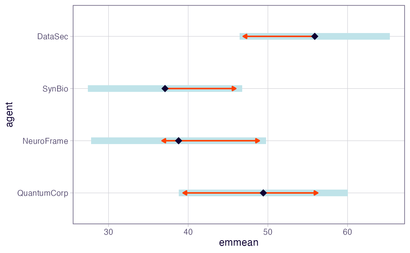
#> 1 QuantumCorp  49.42600
#> 2  NeuroFrame  38.79500
#> 3      SynBio  37.09278
#> 4     DataSec  55.88158

# Change scores
curiosity$change <- curiosity$after6msc - curiosity$baseline
aggregate(change ~ agent, data = curiosity, FUN = mean)
#>         agent     change
#> 1 QuantumCorp -7.8140000
#> 2  NeuroFrame -0.8271429
#> 3      SynBio  6.6805556
#> 4     DataSec -1.7531579

# One-way ANOVA
model <- aov(after6msc ~ agent, data = curiosity)
summary(model)
#>             Df Sum Sq Mean Sq F value Pr(>F)  
#> agent        3   4179  1392.9   3.297 0.0261 *
#> Residuals   62  26194   422.5                 
#> ---
#> Signif. codes:  0 ‘***’ 0.001 ‘**’ 0.01 ‘*’ 0.05 ‘.’ 0.1 ‘ ’ 1

# Post-hoc Tukey comparisons
TukeyHSD(model)
#>   Tukey multiple comparisons of means
#>     95% family-wise confidence level
#> 
#> Fit: aov(formula = after6msc ~ agent, data = curiosity)
#> 
#> $agent
#>                              diff         lwr       upr     p adj
#> NeuroFrame-QuantumCorp -10.631000 -30.7966154  9.534615 0.5091987
#> SynBio-QuantumCorp     -12.333222 -31.3045277  6.638083 0.3240619
#> DataSec-QuantumCorp      6.455579 -12.2874233 25.198581 0.7999409
#> SynBio-NeuroFrame       -1.702222 -21.0395673 17.635123 0.9955329
#> DataSec-NeuroFrame      17.086579  -2.0268356 36.199994 0.0957294
#> DataSec-SynBio          18.788801   0.9399636 36.637639 0.0353590
#> 

# Or with emmeans
if (requireNamespace("emmeans", quietly = TRUE)) {
  library(emmeans)
  emm <- emmeans(model, ~ agent)
  pairs(emm, adjust = "tukey")
  plot(emm, comparisons = TRUE)
}
#> Welcome to emmeans.
#> Caution: You lose important information if you filter this package's results.
#> See '? untidy'
#> 
#> Attaching package: ‘emmeans’
#> The following object is masked from ‘package:RougeLM’:
#> 
#>     nutrition


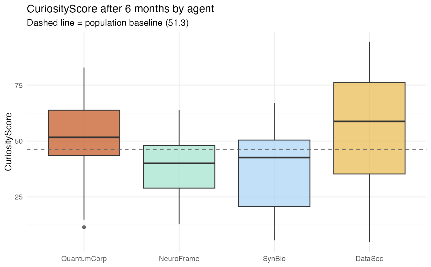
# Visualise distributions
if (requireNamespace("ggplot2", quietly = TRUE)) {
  library(ggplot2)
  ggplot(curiosity,
         aes(x = agent, y = after6msc, fill = agent)) +
    geom_boxplot(alpha = 0.7) +
    geom_hline(yintercept = mean(curiosity$baseline),
               linetype = "dashed", colour = "grey40") +
    scale_fill_manual(values = c(
      "QuantumCorp" = "#c4521a",
      "SynBio"      = "#a8d4f5",
      "DataSec"     = "#e8b84b",
      "NeuroFrame"  = "#9FE1CB"
    )) +
    labs(title    = "CuriosityScore after 6 months by agent",
         subtitle = "Dashed line = population baseline (51.3)",
         x = NULL, y = "CuriosityScore") +
    theme_minimal() +
    theme(legend.position = "none")
}