CuriosityScore dose-response for QuantumCorp's autonomous agent

A simulated dataset of 1,012 WaszKrak residents who interacted with QuantumCorp's autonomous AI agent over a six-month period. For each resident the dataset records their weekly interaction frequency with the agent (dose) and the change in CuriosityScore over the observation period (drop). The dataset is designed to illustrate piecewise (segmented) regression, minimum effective dose analysis, and the detection of a behavioural threshold below which no effect is observed.

The story

The dataset arrived from the same anonymous source as the four-corporation ANOVA data — same metadata stripping, same clean headers, same feeling that someone on the inside was paying attention.

This time it was simpler. Two variables. One thousand and twelve users of QuantumCorp's autonomous agent over six months.

Beta ran the scatter plot first. Old habit.

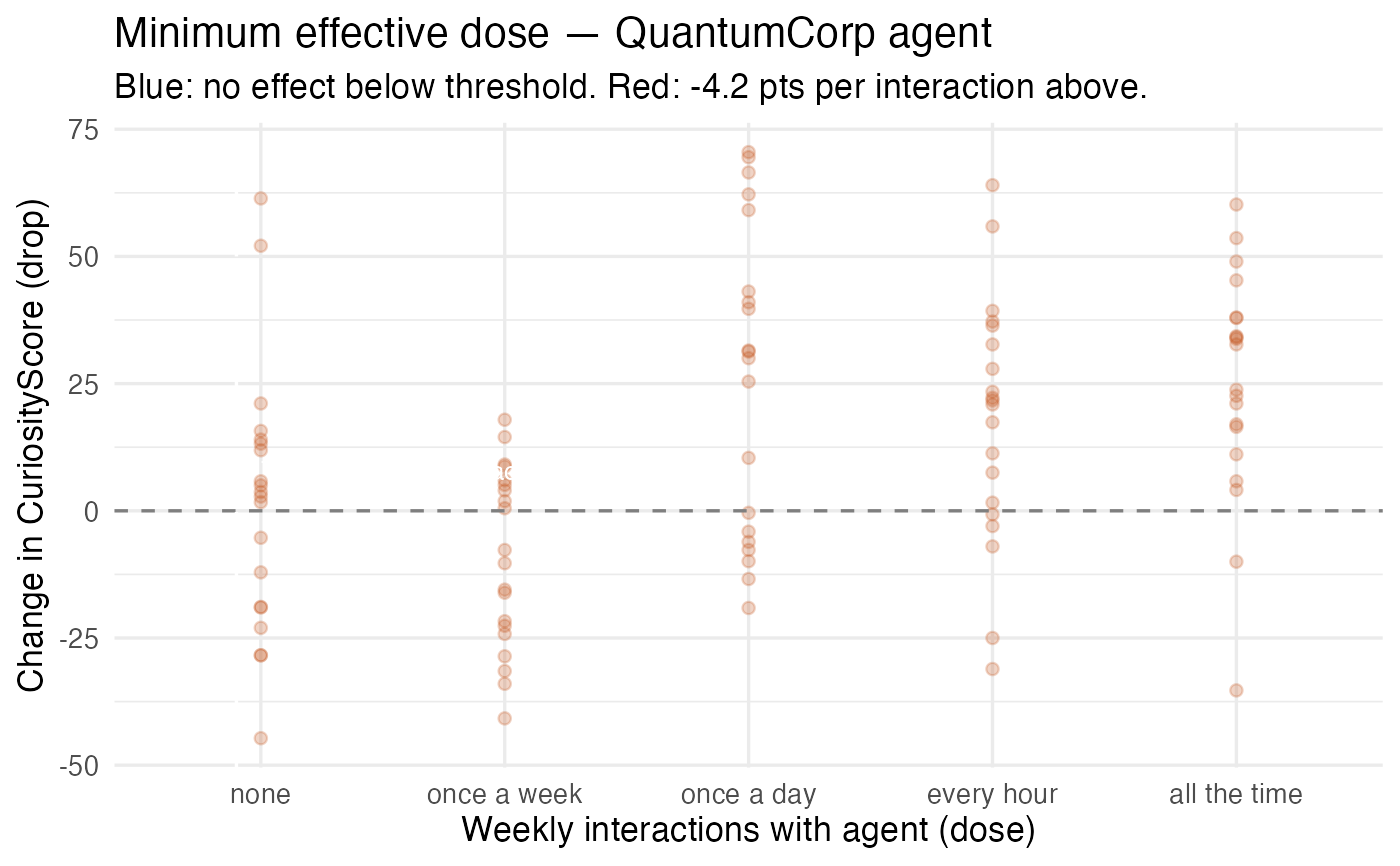
The plot was not linear. It was not even smoothly curved. It was broken. Below a certain frequency threshold, the points scattered randomly around zero — some up, some down, no pattern, no trend. Normal noise. The kind of variation you would expect from life. But somewhere around one interaction per week, the plot changed character entirely. Above that threshold, every single point was negative.

"There's a breakpoint," Bit said.

"Around 0.9 interactions per week," Beta said. She was already fitting the piecewise model. "Below it: slope not different from zero. Flat. No effect. Above it—"

The estimate came back.

Below threshold: $\hat\beta = -0.31$, p = 0.44. Effectively zero.

Above threshold: $\hat\beta = -4.2$ per additional weekly interaction, p < 0.001.

"They found the minimum effective dose," Bit said.

Once a week. Casual enough to feel like nothing. Precise enough to work.

Minimum effective dose

In pharmacology, the minimum effective dose (MED) is the smallest dose required to produce a measurable effect. Here the “dose” is interaction frequency with QuantumCorp's agent, and the “effect” is the reduction in CuriosityScore. The MED is approximately 0.9 interactions per week — just below once weekly.

The threshold was not set at twice a week or daily use. It was set at the frequency that feels casual and natural — like checking the news, like asking a question you would have looked up anyway. The agent's design was not accidental. You do not find a threshold this clean by accident.

Statistical design

The piecewise regression model fits two separate linear segments joined at an estimated breakpoint $x_0$:

$$ \text{drop}_i = \begin{cases} \alpha_1 + \beta_1 \cdot \text{dose}_i + \varepsilon_i & \text{if } \text{dose}_i < x_0 \\ \alpha_2 + \beta_2 \cdot \text{dose}_i + \varepsilon_i & \text{if } \text{dose}_i \geq x_0 \end{cases} $$

The breakpoint $x_0$ can be estimated by the segmented package or by grid search over candidate breakpoints minimising RSS. Below the breakpoint, $\beta_1$ is not significantly different from zero (no effect). Above it, $\beta_2 \approx -4.2$ (each additional weekly interaction reduces CuriosityScore by approximately 4.2 points).

Usage

curiosity_quantum

Format

A data frame with 1,012 rows and 2 variables:

dose: Numeric (0–14). Mean number of interactions with QuantumCorp's autonomous agent per week, averaged over the six-month observation period. An “interaction” is defined as any user-initiated query or agent-initiated notification that received a response within 60 seconds. Values below 0.9 show no significant relationship with drop; values above 0.9 show a strong negative linear relationship. The critical threshold of approximately 0.9 interactions per week corresponds to slightly less than once weekly — a frequency that feels incidental rather than habitual to most users.
drop: Numeric. Change in CuriosityScore over the six-month observation period, defined as CuriosityScore_after - CuriosityScore_before. Negative values indicate a reduction in autonomous information-seeking behaviour. Values near zero indicate no measurable effect of agent exposure. Below the dose threshold of 0.9, drop is distributed approximately as $N(0, \sigma^2)$ — consistent with natural week-to-week variation. Above the threshold, drop is systematically negative with magnitude increasing linearly with dose.

Source

Simulated dataset generated by data-raw/generate_curiosity_quantum.R. The data structure is based on the chapter "The Threshold" in Equations from District 7: A Practical Guide to Linear Models (BetaBit StatPunk universe). All values are fictional.

Examples

data(curiosity_quantum)

# Basic summary
summary(curiosity_quantum)
#>       drop                  dose   
#>  Min.   :-44.70   none        :20  
#>  1st Qu.: -7.70   once a week :20  
#>  Median : 10.75   once a day  :20  
#>  Mean   : 12.11   every hour  :20  
#>  3rd Qu.: 32.70   all the time:20  
#>  Max.   : 70.50                    

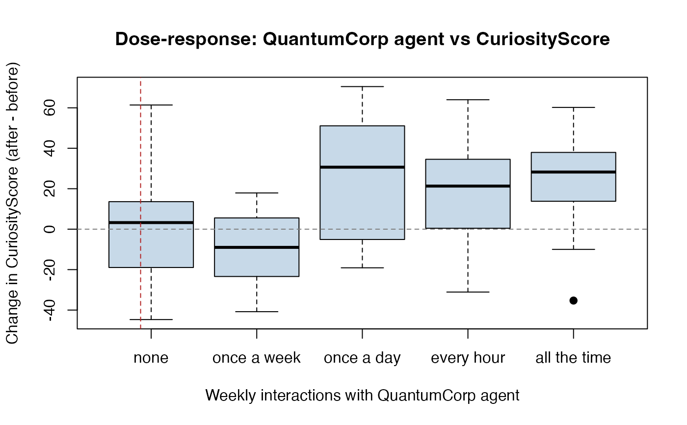
# Scatter plot — the broken relationship
plot(drop ~ dose, data = curiosity_quantum,
     xlab = "Weekly interactions with QuantumCorp agent",
     ylab = "Change in CuriosityScore (after - before)",
     main = "Dose-response: QuantumCorp agent vs CuriosityScore",
     pch  = 19, col = adjustcolor("steelblue", alpha.f = 0.3))
abline(h = 0, lty = 2, col = "grey50")
abline(v = 0.9, lty = 2, col = "firebrick")


# Simple linear model — misses the threshold structure
model_linear <- lm(drop ~ dose, data = curiosity_quantum)
summary(model_linear)
#> 
#> Call:
#> lm(formula = drop ~ dose, data = curiosity_quantum)
#> 
#> Residuals:
#>    Min     1Q Median     3Q    Max 
#> -60.08 -18.49   2.77  14.53  59.97 
#> 
#> Coefficients:
#>                  Estimate Std. Error t value Pr(>|t|)   
#> (Intercept)         1.430      5.485   0.261  0.79488   
#> doseonce a week   -10.695      7.757  -1.379  0.17121   
#> doseonce a day     24.545      7.757   3.164  0.00209 **
#> doseevery hour     16.200      7.757   2.088  0.03944 * 
#> doseall the time   23.350      7.757   3.010  0.00334 **
#> ---
#> Signif. codes:  0 ‘***’ 0.001 ‘**’ 0.01 ‘*’ 0.05 ‘.’ 0.1 ‘ ’ 1
#> 
#> Residual standard error: 24.53 on 95 degrees of freedom
#> Multiple R-squared:  0.2503,	Adjusted R-squared:  0.2187 
#> F-statistic: 7.929 on 4 and 95 DF,  p-value: 1.471e-05
#> 

# Manual piecewise model with known breakpoint at 0.9
curiosity_quantum$above_threshold <- curiosity_quantum$dose >= 0.9
#> Warning: ‘>=’ not meaningful for factors

model_below <- lm(drop ~ dose,
                  data = subset(curiosity_quantum,
                                above_threshold == FALSE))
#> Error in `contrasts<-`(`*tmp*`, value = contr.funs[1 + isOF[nn]]): contrasts can be applied only to factors with 2 or more levels
model_above <- lm(drop ~ dose,
                  data = subset(curiosity_quantum,
                                above_threshold == TRUE))
#> Error in `contrasts<-`(`*tmp*`, value = contr.funs[1 + isOF[nn]]): contrasts can be applied only to factors with 2 or more levels

cat("Below threshold — slope:", round(coef(model_below)["dose"], 3),
    "  p:", round(summary(model_below)$coefficients["dose", 4], 3), "\n")
#> Error: object 'model_below' not found
cat("Above threshold — slope:", round(coef(model_above)["dose"], 3),
    "  p:", round(summary(model_above)$coefficients["dose", 4], 4), "\n")
#> Error: object 'model_above' not found

# Segmented regression — estimate breakpoint automatically
if (requireNamespace("segmented", quietly = TRUE)) {
  library(segmented)
  model_seg <- segmented(
    lm(drop ~ dose, data = curiosity_quantum),
    seg.Z   = ~ dose,
    psi     = 0.9   # starting value for breakpoint
  )
  summary(model_seg)
  plot(model_seg, add = TRUE, col = "firebrick", lwd = 2)
}

# Visualise with ggplot2
if (requireNamespace("ggplot2", quietly = TRUE)) {
  library(ggplot2)
  ggplot(curiosity_quantum,
         aes(x = dose, y = drop)) +
    geom_point(alpha = 0.25, colour = "#c4521a") +
    geom_hline(yintercept = 0,   linetype = "dashed", colour = "grey50") +
    geom_vline(xintercept = 0.9, linetype = "dashed", colour = "white") +
    geom_smooth(data = ~ subset(.x, dose <  0.9),
                method = "lm", se = TRUE,
                colour = "#a8d4f5", linewidth = 1.4) +
    geom_smooth(data = ~ subset(.x, dose >= 0.9),
                method = "lm", se = TRUE,
                colour = "#c4521a", linewidth = 1.4) +
    annotate("text", x = 1.0, y = 8,
             label = "Threshold: 0.9 interactions/week",
             colour = "white", hjust = 0, size = 3.5) +
    labs(title    = "Minimum effective dose — QuantumCorp agent",
         subtitle = "Blue: no effect below threshold. Red: -4.2 pts per interaction above.",
         x = "Weekly interactions with agent (dose)",
         y = "Change in CuriosityScore (drop)") +
    theme_minimal(base_size = 13)
}
#> Warning: ‘<’ not meaningful for factors
#> Warning: ‘>=’ not meaningful for factors