6  Two-Way ANOVA and the MobilityScore story

6.1 The Case: Where the Lines Cross

Run, run as fast as you can

The message came in plain text. No encryption, no onion routing, no attempt to hide.

My name is Marek Kowalski. I live in District 7. I am 43. My daughter is 24. We both applied for mobility reclassification last month. She was approved. I was not. I want to know why the same district produces different people.

“He signed his real name,” Bit said, reading it twice.

“He doesn’t care,” Beta said. “Or he doesn’t know enough yet to be afraid.”

She wrote back in twenty minutes and asked for whatever he could gather: his own public scoring profile, his daughter’s, and anyone else willing to share. But Marek’s building was not the whole city, and Beta knew better than to diagnose a system from one stairwell. She widened the request through the few clinic contacts she trusted, and three days later four hundred and twelve records arrived. Not District 7 alone. Three districts: the struggling 7, the middling 12, and the comfortable 23. Each resident tagged with gender, an age band, junior, mid, or senior, and a MobilityScore pulled from the public allocation feed. If the reclassification algorithm was doing something to people like Marek, it would show up as a pattern across all three, not just in his corridor.

She started where everyone starts, with the obvious suspects. Did men and women score differently? She pooled every resident and compared. The gap was almost nothing, a whisper of a difference, and the test waved it away. Gender, on its own, explained essentially none of the variation in MobilityScore. Then age, on its own: junior versus mid versus senior, pooled across gender and district. Also nothing. The age bands drifted around a common center, and the test could not tell them apart either.

Two dead ends. On paper, District life looked gender-blind and age-blind, exactly the kind of result the reclassification board would love to quote.

“So there’s nothing,” Bit said.

“So there’s nothing on the surface,” Beta said. She did not believe it, because Marek and his daughter were the same district, the same building, the same blood, and one was approved and one was not. A difference had to live somewhere. If it was not in gender alone and not in age alone, then maybe it only existed in the two of them together, the way a lock does not open to either half of a key.

So she built the model that let gender and age interact rather than sit side by side. And this time something surfaced. The interaction term was significant, modestly but unmistakably. Adding it improved the model in a way that chance could not comfortably explain, even though neither factor had meant anything alone. She pulled the estimated marginal means and laid them out as a two-by-two grid, and the shape underneath finally showed itself.

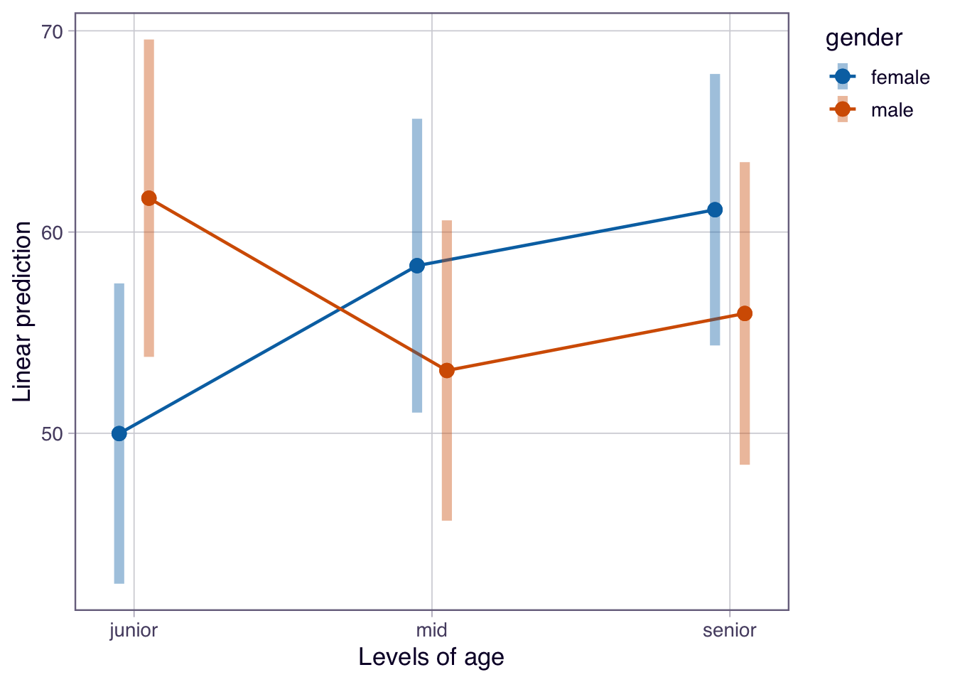
Among the juniors, men scored well above women, better than sixty against an even fifty. But that ordering did not hold. By the mid band the women had pulled ahead, and among seniors they stayed ahead. The lines for the two genders did not run parallel and they did not merely drift apart. They crossed. Somewhere between junior and mid, in the pooled picture, the advantage flipped from men to women.

“Plot it,” Bit said quietly.

The interaction plot appeared: two lines starting apart at junior, one falling, one rising, scissoring past each other on the way to mid. The kind of picture that makes a statistician sit still, not because it is mathematically strange but because it means every headline number about gender in these districts, every pooled average, was true and useless at once. The main effects were null precisely because the two halves of the crossing cancelled when you flattened them together.

“That’s the whole trick,” Beta said. “Average a rise and a fall and you get a flat line. The board runs the one-factor tests, sees nothing, and calls the system fair. The unfairness doesn’t disappear. It just hides in the interaction, where they never look.”

But she was still uneasy, because Marek was District 7 and this was three districts stirred together. A crossing in the pooled data did not tell her where it happened, or whether it was one district dragging the average or all three behaving alike. So she added the third factor. District, with all of its interactions, gender by age by district, free to behave differently in each place.

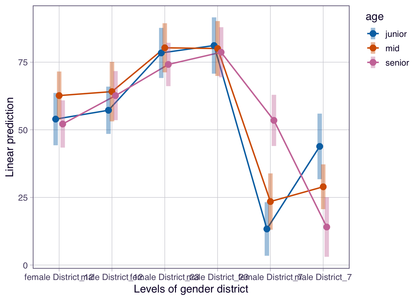
The moment district entered, the model changed character entirely. It mattered enormously, past any doubt, and the three-way interaction with it was strongly significant. When she split the means by district, the reason was brutal and specific. In the comfortable districts the age-and-gender pattern was mild, scores high and the two genders tracking each other across the bands. But District 7 was a different country. There, the women rose steadily with age while the men collapsed: young men scoring in the forties and sinking into the teens by senior, young women starting near the bottom and climbing past fifty. The clean crossing she had seen in the pooled data was mostly District 7 shouting through the average. Marek’s district was not an example of the pattern. It was the source of it.

Beta sat with the three-way means for a while before she wrote anything.

The questions were now sharp enough to answer one at a time, in order, the way the model had been built. Why did gender and age each look meaningless alone, and what does it mean that a factor can vanish in a main-effect test yet return through an interaction? Was the gender-by-age interaction real, or within reach of chance, and how would comparing the additive model against the interaction model settle it? And once district entered, did the gender-and-age story hold everywhere, or did the three-way test confirm what the means whispered, that District 7 alone bent the curve? Only after those, she thought, could she write the second document. The one without notation. The one for Marek, that would explain why the same district produced two different people, and why the machine had been sure it was measuring mobility when it was only ever photocopying the past.

6.2 The Formula: Two-Way ANOVA and Interaction Effects

In the story from the previous section, Beta encountered a result that a simpler analysis would have missed entirely. The effect of gender on MobilityScore was not significant when examined alone. The effect of age was significant. But neither effect told the complete story, only the interaction between them revealed the structure underneath. This is the central insight of two-way ANOVA: main effects can be misleading when an interaction is present, so we need methods to detect and model interactions.

6.2.1 The Model

In the case of one-way analysis of variance, we examined relationships between groups of objects defined by one categorical variable. Two-way analysis of variance allows exmining the relationship between a quantitative variable \(y\) and two categorical variables, which we’ll denote A and B in what follows. We can consider different models for such a relationship; below we’ll describe the most popular ones: additive main effects with and without interaction.

Assume that variable A can occur at \(k\) levels and variable B at \(r\) levels. The analysis of variance model is as follows:

\[ y_{ijm} \sim \mathcal{N}(\mu_{i,j}, \sigma^2), \quad 1 \leq i \leq k, \quad 1 \leq j \leq r, \quad 1 \leq m \leq n_{i,j}. \tag{6.1}\]

where response variable \(y|A=i,B=j\) has a normal distribution with variance \(\sigma^2\) and mean \(\mu_{i,j}\), and \(n_{i,j}\) is the number of observations for which variable A takes value \(i\) and variable B takes value \(j\).

If \(n_{i,j}\) is the same in each group, we speak of a balanced design; otherwise, an unbalanced design.

Hypotheses posed in two-way analysis of variance concern the values of means \(\mu_{i,j}\), of which there are \(k r\). Let’s present them in a table together with marginal means.

\[ \begin{array}{llll|l} \mu_{1,1} & \mu_{1,2} & \cdots & \mu_{1,r} & \mu_{1,.} \\ \mu_{2,1} & \mu_{2,2} & \cdots & \mu_{2,r} & \mu_{2,.} \\ \cdots & \cdots & \cdots & \cdots & \cdots \\ \mu_{k,1} & \mu_{k,2} & \cdots & \mu_{k,r} & \mu_{k,.} \\ \hline \mu_{.,1} & \mu_{.,2} & \cdots & \mu_{.,r} & \mu \\ \end{array} \tag{6.2}\]

If the design is balanced, that is, counts in each group are equal to each other, then marginal means are arithmetic means of means in corresponding groups:

\[ \mu_{i,.} = \sum_{j=1}^r \mu_{i,j} / r, \]

and

\[ \mu_{.,j} = \sum_{i=1}^k \mu_{i,j} / k. \]

In analysis of variance, different parameterizations are usually used in which means \(\mu_{i,j}\) are expressed by effects \(\mu\), \(\alpha_1\), \(\alpha_2\), …, \(\alpha_k\), \(\beta_1\), …, \(\beta_r\), \(\gamma_{1,1}\), …, \(\gamma_{k,r}\). These effects are called respectively: grand mean, main additive effects of the first variable, main additive effects of the second variable, and interaction effects (each group of effects is denoted by a different Greek letter).

Using these effects, model Equation 6.1 can be written as:

\[ y_{ijk} = \mu + \alpha_i + \beta_j + (\alpha\beta)_{ij} + \varepsilon_{ijk} \tag{6.3}\]

where:

  • \(\mu\) is the grand mean,
  • \(\alpha_i\) is the main effect of factor \(A\) at level \(i\),
  • \(\beta_j\) is the main effect of factor \(B\) at level \(j\),
  • \((\alpha\beta)_{ij}\) is the interaction effect for pair of factors \(i,j\),
  • \(\varepsilon_{ijk} \sim \mathcal{N}(0, \sigma^2)\) is the random noise for observation \(k\) in cell \((i,j)\).

The interaction term \((\alpha\beta)_{ij}\) captures what cannot be explained by the main effects alone, the degree to which the effect of factor \(A\) depends on the level of factor \(B\), and vice versa.

Note, that the number of parameters in the description Equation 6.3 (that is \((k+1)*(r+1)\)) is larger than number of observed values (that is \(k*r\) means), some constraints must be imposed on the new parameters to make them identifiable. A one possible choice is

  • either the constraint:

\[ \sum_{i=1}^k \alpha_i = 0,\quad \sum_{j=1}^r \beta_j = 0,\quad \forall_i \quad \sum_{j=1}^r \gamma_{i,j} = 0,\quad \forall_j \quad \sum_{i=1}^k \gamma_{i,j} = 0. \]

  • or the constraint:

\[\begin{equation} \alpha_1=0, \quad \beta_1=0, \quad \forall_i \quad \gamma_{i,1}=0, \quad \forall_j \quad \gamma_{1,j}=0. \end{equation}\]

The latter is used by default in many statistical packages so we will work with this one. With such constraints, the matrix of means Equation 6.2 can be presented in a new parameterization unambiguously.

By interaction, we mean the deviation of mean \(\mu_{i,j}\) from the additive influence of group \(i\) of the first variable and group \(j\) of the second variable. A model without interaction differs from a model with interaction in that in the case of a model without interaction, it’s assumed that all values \(\forall_{i,j} \gamma_{i,j}=0\). The occurrence of an interaction effect doesn’t mean the model isn’t linear.

Translating the above description into the language of linear models, we’ll consider a linear model of the form:

\[ y = X \beta + \varepsilon, \]

in which vector \(\beta = (\mu, \alpha_2, \ldots, \alpha_k, \beta_2, \ldots, \beta_r, \gamma_{2,2}, \ldots, \gamma_{kr})\), and matrix \(X\) is a matrix of indicators of individual factors.

For example, assume we have a set of twelve observations and three variables: one quantitative \(y\) and two categorical \(x_1\) and \(x_2\). Assume that variable \(x_1\) occurs at two levels: C or D, and the number of occurrences of each level is balanced and equals six occurrences. In other words, the variable \(x_1=c(C, C, C, C, C, C, D, D, D, D, D, D)\) describes two six-element groups. Assume that variable \(x_2\) occurs at three equally frequent levels: Q, R, or S. In other words, the variable \(x_2=c(Q, Q, R, R, S, S, Q, Q, R, R, S, S)\) describes three four-element groups.

The formula y~x1+x2 describes a two-way analysis of variance model without interaction. The corresponding matrix notation of the model is as follows:

\[ \begin{bmatrix} y_{1,1,1} \\ y_{1,1,2} \\ y_{1,2,1} \\ y_{1,2,2} \\ y_{1,3,1} \\ y_{1,3,2} \\ y_{2,1,1} \\ y_{2,1,2} \\ y_{2,2,1} \\ y_{2,2,2} \\ y_{2,3,1} \\ y_{2,3,2} \end{bmatrix} = \begin{bmatrix} 1 & 0 & 0 & 0 \\ 1 & 0 & 0 & 0 \\ 1 & 0 & 1 & 0 \\ 1 & 0 & 1 & 0 \\ 1 & 0 & 0 & 1 \\ 1 & 0 & 0 & 1 \\ 1 & 1 & 0 & 0 \\ 1 & 1 & 0 & 0 \\ 1 & 1 & 1 & 0 \\ 1 & 1 & 1 & 0 \\ 1 & 1 & 0 & 1 \\ 1 & 1 & 0 & 1 \end{bmatrix} \begin{bmatrix} \mu\\ \alpha_2\\ \beta_2\\ \beta_3 \end{bmatrix} + \begin{bmatrix} \varepsilon_{1,1,1} \\ \varepsilon_{1,1,2} \\ \varepsilon_{1,2,1} \\ \varepsilon_{1,2,2} \\ \varepsilon_{1,3,1} \\ \varepsilon_{1,3,2} \\ \varepsilon_{2,1,1} \\ \varepsilon_{2,1,2} \\ \varepsilon_{2,2,1} \\ \varepsilon_{2,2,2} \\ \varepsilon_{2,3,1} \\ \varepsilon_{2,3,2} \end{bmatrix}. \tag{6.4}\]

The formula with interaction y~x1*x2 is equivalent to the formula y~x1+x2+x1:x2. Both describe a two-way analysis of variance model with interaction. The corresponding matrix notation is as follows:

\[ \begin{bmatrix} y_{1,1,1} \\ y_{1,1,2} \\ y_{1,2,1} \\ y_{1,2,2} \\ y_{1,3,1} \\ y_{1,3,2} \\ y_{2,1,1} \\ y_{2,1,2} \\ y_{2,2,1} \\ y_{2,2,2} \\ y_{2,3,1} \\ y_{2,3,2} \end{bmatrix} = \begin{bmatrix} 1 & 0 & 0 & 0 & 0 & 0 \\ 1 & 0 & 0 & 0 & 0 & 0 \\ 1 & 0 & 1 & 0 & 0 & 0 \\ 1 & 0 & 1 & 0 & 0 & 0 \\ 1 & 0 & 0 & 1 & 0 & 0 \\ 1 & 0 & 0 & 1 & 0 & 0 \\ 1 & 1 & 0 & 0 & 0 & 0 \\ 1 & 1 & 0 & 0 & 0 & 0 \\ 1 & 1 & 1 & 0 & 1 & 0 \\ 1 & 1 & 1 & 0 & 1 & 0 \\ 1 & 1 & 0 & 1 & 0 & 1 \\ 1 & 1 & 0 & 1 & 0 & 1 \end{bmatrix} \begin{bmatrix} \mu\\ \alpha_2\\ \beta_2\\ \beta_3\\ \gamma_{2,2}\\ \gamma_{2,3} \end{bmatrix} + \begin{bmatrix} \varepsilon_{1,1,1} \\ \varepsilon_{1,1,2} \\ \varepsilon_{1,2,1} \\ \varepsilon_{1,2,2} \\ \varepsilon_{1,3,1} \\ \varepsilon_{1,3,2} \\ \varepsilon_{2,1,1} \\ \varepsilon_{2,1,2} \\ \varepsilon_{2,2,1} \\ \varepsilon_{2,2,2} \\ \varepsilon_{2,3,1} \\ \varepsilon_{2,3,2} \end{bmatrix}, \tag{6.5}\]

where \((y_{1,1,1}, y_{1,1,2}, \ldots, y_{2,3,1}, y_{2,3,2})\) is a twelve-element vector with measurements of trait \(y\), and \((\varepsilon_{1, 1,1}, \varepsilon_{1, 1,2}, \ldots, \varepsilon_{2,3,1}, \varepsilon_{2,3,2})\) is a twelve-element vector corresponding to random disturbance \(\varepsilon \sim \mathcal{N}(0, I_{12\times 12}\sigma^2)\).

6.2.2 It’s all about testing

For a two-way ANOVA three sets of hypotheses can be considered. We’ll present them using the above parameterization.

  • Hypotheses related to main effects of variable \(A\). Does the mean of the response variable differ significantly across the possible values of variable \(A\) (similar to one-way ANOVA)?

\[H_0: \alpha_1 = \alpha_2 = \cdots = \alpha_I = 0 \tag{6.6}\]

\[H_A: \text{at least one } \alpha_i \neq 0\]

  • Hypotheses related to main effects of variable \(B\). Does the mean of the response variable differ significantly across the possible values of variable \(B\) (similar to one-way ANOVA but for the second variable)?

\[H_0: \beta_1 = \beta_2 = \cdots = \beta_J = 0 \tag{6.7}\]

\[H_A: \text{at least one } \beta_j \neq 0\]

  • Hypotheses related to interaction effects between variables \(A\) and \(B\). Does the mean mean differs from the value that would have been estimated without taking the interaction into account?

\[H_0: (\alpha\beta)_{ij} = 0 \quad \text{for all } i, j \tag{6.8}\]

\[H_A: \text{at least one } (\alpha\beta)_{ij} \neq 0\]

Each of these hypotheses concerns a set of effects; each can be verified using the likelihood ratio test presented in Section 3.5.4.

The typical testing procedure begins with interactions. If there are no interactions, we can test each hypothesis regarding the main effects independently. However, if interactions are present, we know that both variables \(A\) and \(B\) are significant.

6.3 The Terminal: Two-Way ANOVA in R

The dataset used in this section comes from the RougeLM package. The mobility dataset contains 412 District 7 residents with their score (MobilityScore), gender, age group, and district.

library("RougeLM")
head(mobility)
     district gender    age score
1  District_7   male    mid    72
2 District_23   male senior    49
3 District_12   male senior    57
4  District_7   male    mid    14
5 District_23 female junior    68
6  District_7 female junior    41

head() confirms the structure: each row is one resident. score is the continuous response variable. gender and age are the two categorical factors for the two-way ANOVA. district will be introduced as a third factor in the extended models later in this section.


6.3.1 Show me the data

With two categorical factors and one continuous response, the first visualisation should show all three simultaneously. Boxplot will do the job here.

library("ggplot2")

ggplot(mobility, aes(x = age, y = score, color = gender)) +
  geom_boxplot() 
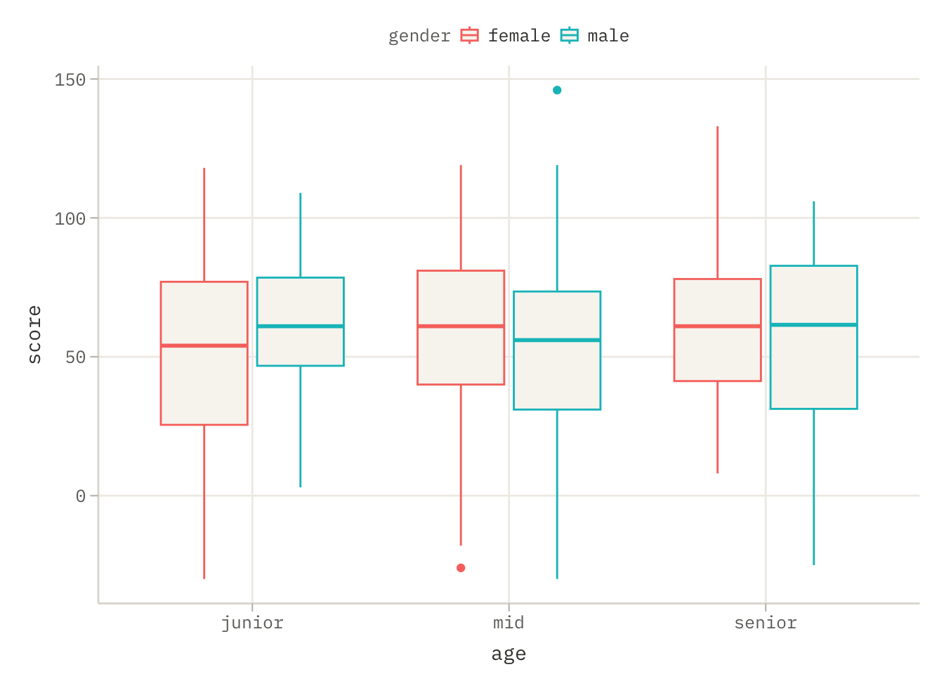
Figure 6.1: Distribution of MobilityScore by age group (x-axis) and gender (colour). Each box shows the interquartile range with the median as a horizontal line.

ggplot(mobility, aes(x = age, y = score, color = gender)) initialises the plot with age on the x-axis, score on the y-axis, and gender mapped to colour. Mapping gender to colour rather than to x places the two gender groups side by side within each level of age, making the gender difference visually immediate.

geom_boxplot() draws one box per combination of age and gender. Because gender is mapped to colour, the two boxes within each age level are automatically distinguished by fill and outline colour.

This time, the chart shows that there may be some small difference between MobilityScore in the junior category, but is it significant?


6.3.2 Group means table

A mean table makes the pattern visible in numbers before any formal test.

library("dplyr")
library("tidyr")

mobility |>
  group_by(gender, age) |>
  summarise(avg_score = mean(score)) |>
  pivot_wider(names_from = age, values_from = avg_score)
# A tibble: 2 × 4
# Groups:   gender [2]
  gender junior   mid senior
  <fct>   <dbl> <dbl>  <dbl>
1 female   50.0  58.3   61.1
2 male     61.7  53.1   56.0
Table 6.1: A table showing the mean values for each combination of gender and age variables

group_by(gender, age) partitions the data by all combinations of the two factors — one group per cell of the two-way design. summarise(avg_score = mean(score)) computes the mean score within each cell and collapses the group to a single row. At this point the result is a long data frame with one row per gender-age combination.

pivot_wider(names_from = age, values_from = avg_score) reshapes the long result into a wide table. names_from = age takes the levels of age and creates one column per level; values_from = avg_score fills those columns with the corresponding means. The result is a compact two-by-two table with gender as rows and age groups as columns, the standard layout for inspecting a two-way interaction.


6.3.3 Model without interaction

Let’s start with a model for two variables without interaction. This will correspond to an \(X\) matrix with three components, as shown in Equation 6.4.

The first step is to estimate the coefficients, which will be \(1+(r-1)+(k-1)\).

model_mob_01 <- lm(score ~ gender + age, data = mobility)
model_mob_01$coefficients
Listing 6.1: Coefficients in the ANOVA model for the variables ‘gender’ and ‘age’, excluding interactions.
(Intercept)  gendermale      agemid   agesenior 
55.49590528  0.03366716  0.26865166  3.29989180 

lm(score ~ gender + age, data = mobility) fits the additive two-way model. The + operator in the formula specifies that both gender and age are included as main effects but their interaction is not. The model assumes that the effect of gender on score is the same regardless of age group, and vice versa, a strong assumption that will be tested below.

model_mob_01$coefficients extracts only the coefficient vector from the fitted model object, without the standard errors, t-values, or p-values that summary() would produce. This is useful for a quick look at the estimated effects before examining the full inferential output. Each named element corresponds to one column of the design matrix: (Intercept) is the mean of the reference cell, and the remaining coefficients are deviations from that reference.

Do these variables matter? In a model without interactions, we can test hypotheses for the main effects, that is Equation 6.6 and Equation 6.7.

anova(model_mob_01)
Analysis of Variance Table

Response: score
           Df Sum Sq Mean Sq F value Pr(>F)
gender      1      0    0.45  0.0005 0.9829
age         2    951  475.50  0.4871 0.6148
Residuals 408 398278  976.17               
Table 6.2

anova() applied to a single lm object produces a sequential (Type I) analysis of variance table. The predictors are tested in the order they appear in the formula: gender is tested first, then age conditional on gender. Each row reports the sum of squares, degrees of freedom, mean square, F-statistic, and p-value for the effect of adding that term to the model. A significant F-value for a term means that adding it improved model fit beyond what chance would predict.


6.3.4 Model with interaction

Let’s add to this model effect for possible interactions. This will correspond to an X matrix with four components, as shown in Equation 6.5.

model_mob_02 <- lm(score ~ gender * age, data = mobility)
model_mob_02$coefficients
Listing 6.2: Coefficients in the ANOVA model for the variables ‘gender’ and ‘age’, including interactions.
         (Intercept)           gendermale               agemid 
           49.985075            11.698259             8.343497 
           agesenior    gendermale:agemid gendermale:agesenior 
           11.124681           -16.907427           -16.853469 

lm(score ~ gender * age, data = mobility) fits the interaction model. The * operator expands to gender + age + gender:age — it automatically includes both main effects and their interaction term. The interaction term gender:age captures any additional effect that cannot be accounted for by the main effects alone: the degree to which the gender gap in score differs between age groups.

In the coefficient vector, the interaction coefficient gendermale:agesenior measures how much the effect of being male changes when moving from the younger to the older age group, or equivalently, how much the age effect changes when moving from female to male.

Do these interactions matter? In this model we can additionally test hypotheses Equation 6.8 (last row).

anova(model_mob_02)
Analysis of Variance Table

Response: score
            Df Sum Sq Mean Sq F value  Pr(>F)  
gender       1      0    0.45  0.0005 0.98283  
age          2    951  475.50  0.4924 0.61150  
gender:age   2   6232 3116.21  3.2271 0.04069 *
Residuals  406 392045  965.63                  
---
Signif. codes:  0 '***' 0.001 '**' 0.01 '*' 0.05 '.' 0.1 ' ' 1
Table 6.3

The ANOVA table above a third row for the interaction term gender:age shows a significant p-value here indicates that the variables ‘age’ and ‘gender’ may have a weak but statistically significant impact on the MobilityScore, even if these relationships are not apparent when each variable is considered in isolation.


6.3.5 Comparing models with main and and interaction effects

We can also test hypothesis Equation 6.8 independently of the others by directly comparing the two models, with and without interaction. As they are nested, we can use the likelihood ratio test. The result will be the same as in Table 6.3

anova(model_mob_01, model_mob_02)
Analysis of Variance Table

Model 1: score ~ gender + age
Model 2: score ~ gender * age
  Res.Df    RSS Df Sum of Sq      F  Pr(>F)  
1    408 398278                              
2    406 392045  2    6232.4 3.2271 0.04069 *
---
Signif. codes:  0 '***' 0.001 '**' 0.01 '*' 0.05 '.' 0.1 ' ' 1
Table 6.4

anova() with two model objects performs a likelihood ratio (F) test comparing the smaller nested model against the larger one. model_mob_01 is nested within model_mob_02, it is model_mob_02 with the interaction coefficient constrained to zero. The test asks whether adding the interaction term significantly improves fit.

The output table has one row per model. Res.Df is the residual degrees of freedom, RSS the residual sum of squares, Df the difference in the number of parameters, Sum of Sq the reduction in RSS from adding the interaction, F the F-statistic, and Pr(>F) the p-value. If Pr(>F) is below \(\alpha\), the interaction model is preferred over the additive model.


6.3.6 Estimated marginal means

The coefficients estimated in the linear model Listing 6.1 or Listing 6.2 are not marginal means, but rather a default parameterisation that ensures the effect of the first factor is the reference effect. In certain applications, we may wish to estimate the marginal means. To do this, we can use the package emmeans. Let’s look at an example

library("emmeans")

emm <- emmeans(model_mob_02, ~ gender + age)
emm
 gender age    emmean   SE  df lower.CL upper.CL
 female junior   50.0 3.80 406     42.5     57.4
 male   junior   61.7 4.01 406     53.8     69.6
 female mid      58.3 3.71 406     51.0     65.6
 male   mid      53.1 3.80 406     45.7     60.6
 female senior   61.1 3.43 406     54.4     67.9
 male   senior   56.0 3.83 406     48.4     63.5

Confidence level used: 0.95 
Table 6.5: Empirical means for the model with two variables: age and gender

emmeans() from the emmeans package computes estimated marginal means (EMMs), the model-predicted mean score for each combination of gender and age, adjusted for any other terms in the model. The formula ~ gender * age specifies which factors to compute means for.

The output table shows emmean (the point estimate), SE (its standard error), df (degrees of freedom used for inference), and lower.CL / upper.CL (the 95% confidence interval bounds). These are the quantities that post-hoc pairwise comparisons are built from.

emmip(model_mob_02, gender ~ age, CIs = TRUE)
Figure 6.2: Interaction plot from emmeans::emmip(). Each line connects the estimated marginal means for one gender across the two age groups. Lines that are not parallel indicate an interaction; crossing lines indicate a disordinal interaction where the ranking of groups reverses between age categories. Confidence intervals are shown as shaded bands.

emmip() produces an interaction plot directly from a fitted model. The formula gender ~ age places age on the x-axis and draws one line per level of gender. CIs = TRUE adds confidence intervals around each estimated marginal mean as error bars or shaded bands. Unlike a raw data plot, emmip() plots model-estimated means — they account for the model structure rather than simply averaging the raw data within cells.


6.3.7 Three-way model with district

In a similar way to the case of two variables, the ANOVA model can be generalised to three or more variables. In each case, we can consider only the additive effects, all interactions, or only selected interactions. Below, we will practice this with three variables.

6.3.8 Show me the data

With three categorical factors and one continuous response we still can show all four variables simultaneously.

library("ggplot2")

ggplot(mobility, aes(x = age, y = score, color = gender)) +
  geom_boxplot() +
  facet_wrap(~district)
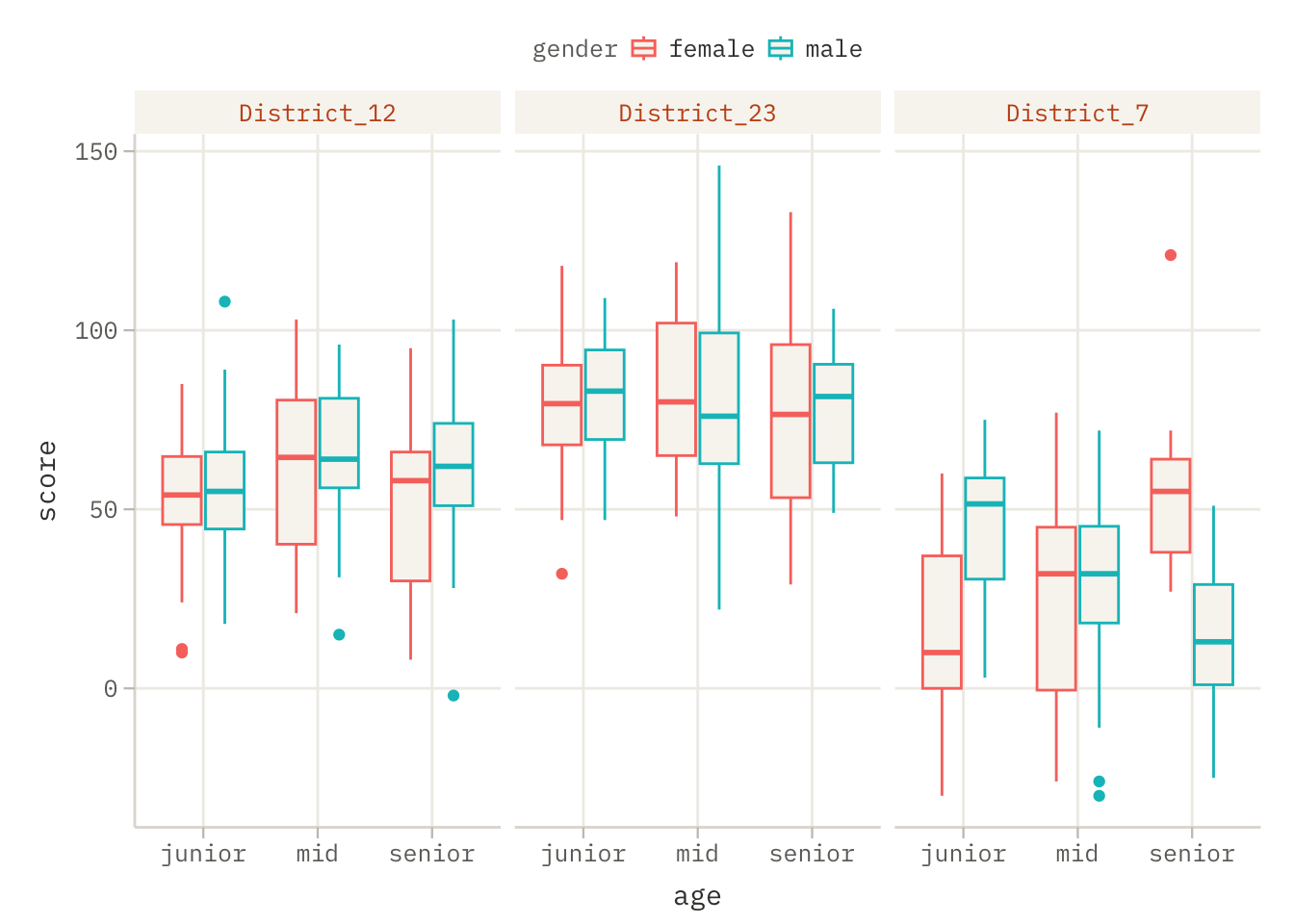
Figure 6.3: Distribution of MobilityScore by age group (x-axis) and gender (colour) within each district (facet). Each box shows the interquartile range with the median as a horizontal line. Examining the plot before fitting any model reveals whether the gender difference appears consistent across age groups or whether it reverses — the hallmark of a disordinal interaction.

The plot is constructed in a similar way to Figure 6.1, but we added facet_wrap(~district) to split the plot into one panel per district. This allows the relationship between age, gender, and score to be examined separately within each district without fitting a model, if the interaction pattern looks different across panels, a district-by-gender or district-by-age interaction may be present in the data.

This time, the chart shows that in District 7, not only is the average MobilityScore different, but the relative relationship between the averages for the two genders also differs from that in other districts.


6.3.9 Group means table

Let’s replicate the mean table with an additional variable district.

library("dplyr")
library("tidyr")

mobility |>
  group_by(district, gender, age) |>
  summarise(avg_score = mean(score)) |>
  pivot_wider(names_from = age, values_from = avg_score)
# A tibble: 6 × 5
# Groups:   district, gender [6]
  district    gender junior   mid senior
  <fct>       <fct>   <dbl> <dbl>  <dbl>
1 District_12 female   54.0  62.7   52.1
2 District_12 male     57.2  64.1   62.6
3 District_23 female   78.4  80.3   74.2
4 District_23 male     81.2  80.0   78.7
5 District_7  female   13.3  23.5   53.5
6 District_7  male     43.9  28.9   14.1
Table 6.6: A table showing the mean values for each combination of district, gender and age variables

6.3.10 Three-way ANOVA model with and without interactions

In a similar way to the two-way ANOVA model, we can add further variables to check whether they have an effect on the dependent variable.

model_mob_05 <- lm(score ~ district + gender + age, data = mobility)
model_mob_06 <- lm(score ~ district * gender * age, data = mobility)

model_mob_05 adds district as an additive main effect alongside gender and age. The + operator means district shifts the intercept, each district has a different baseline score, but the effects of gender and age are assumed identical across districts.

model_mob_06 includes all interactions via *, allowing the gender and age effects to vary freely across districts.

6.3.11 Comparing models

Now that we have fitted models, we can carry out a wide variety of tests. In the case of three variables, are the interactions statistically significant, or is a description using additive effects sufficient?

anova(model_mob_05, model_mob_06)
Analysis of Variance Table

Model 1: score ~ district + gender + age
Model 2: score ~ district * gender * age
  Res.Df    RSS Df Sum of Sq      F    Pr(>F)    
1    406 239177                                  
2    394 209834 12     29343 4.5914 5.679e-07 ***
---
Signif. codes:  0 '***' 0.001 '**' 0.01 '*' 0.05 '.' 0.1 ' ' 1

Oh, they are important! Good to know.

And is the ‘district’ statistically significant?

anova(model_mob_02, model_mob_06)
Analysis of Variance Table

Model 1: score ~ gender * age
Model 2: score ~ district * gender * age
  Res.Df    RSS Df Sum of Sq      F    Pr(>F)    
1    406 392045                                  
2    394 209834 12    182211 28.511 < 2.2e-16 ***
---
Signif. codes:  0 '***' 0.001 '**' 0.01 '*' 0.05 '.' 0.1 ' ' 1

Without a shadow of a doubt.

6.3.12 Estimated marginal means

As with the two-way analysis model, we can display the marginal means, together with their confidence intervals, both numerically and on a graph, to illustrate visually what interactions we expect.

emm <- emmeans(model_mob_06, ~ district * gender * age)
emm
 district    gender age    emmean   SE  df lower.CL upper.CL
 District_12 female junior   54.0 4.92 394    44.28     63.6
 District_23 female junior   78.4 4.71 394    69.16     87.7
 District_7  female junior   13.3 5.04 394     3.43     23.2
 District_12 male   junior   57.2 4.44 394    48.49     66.0
 District_23 male   junior   81.2 5.29 394    70.75     91.6
 District_7  male   junior   43.9 6.17 394    31.73     56.0
 District_12 female mid      62.7 4.53 394    53.76     71.6
 District_23 female mid      80.3 4.62 394    71.25     89.4
 District_7  female mid      23.5 5.29 394    13.06     33.9
 District_12 male   mid      64.1 5.60 394    53.11     75.1
 District_23 male   mid      80.0 5.16 394    69.90     90.2
 District_7  male   mid      28.9 4.21 394    20.65     37.2
 District_12 female senior   52.1 4.44 394    43.42     60.9
 District_23 female senior   74.2 4.08 394    66.14     82.2
 District_7  female senior   53.5 4.81 394    44.02     62.9
 District_12 male   senior   62.6 4.62 394    53.57     71.7
 District_23 male   senior   78.7 4.71 394    69.41     87.9
 District_7  male   senior   14.1 5.60 394     3.05     25.1

Confidence level used: 0.95 
Table 6.7: Empirical means for the model with three variables: district, age and gender
emmip(model_mob_06, age ~ gender * district, CIs = TRUE)
Figure 6.4: Interaction plot for the three-way model: estimated marginal means of MobilityScore by gender and district (x-axis grouped by district), with separate lines for each age group. A three-way interaction would appear as the age-group lines having different shapes across the district panels.

The formula age ~ gender * district in emmip() places the gender * district combination on the x-axis — one tick per gender-district cell — and draws one line per level of age. With two levels of gender, three levels of district, and two levels of age, the plot shows twelve estimated means connected by two lines, one per age group. Comparing the slope of the age lines across districts reveals whether the age effect is consistent across districts or whether district moderates it.

Clearly, the situation in District 7 is different from that in the other districts.


6.4 Exercises

6.4.1 Exercise 1: Reading the two-way ANOVA table

Beta has fitted two models to the mobility dataset:

model_mob_01 <- lm(score ~ gender + age, data = mobility)
model_mob_02 <- lm(score ~ gender * age, data = mobility)

anova(model_mob_01)
anova(model_mob_02)

(a) The additive model model_mob_01 has two rows in its ANOVA table: gender and Residuals. How many rows does the interaction model model_mob_02 have, and what are they? Write down the corresponding null hypothesis for each non-residual row.

(b) In anova(model_mob_01), the gender row is tested first, before age. Explain why the order of terms in the formula matters for the sequential (Type I) sum of squares used by anova(). What would change if you fitted lm(score ~ age + gender, data = mobility) instead?

(c) The interaction term gender:age is significant in anova(model_mob_02). What does this tell you about the parallel-slopes assumption of the additive model? In one sentence, explain why a significant interaction means that the main effect of gender alone is an incomplete — and potentially misleading — summary of the data.


6.4.2 Exercise 2: The design matrix for two factors

head(model.matrix(score ~ gender * age, data = mobility))

(a) Run the command above. How many columns does the design matrix have? Identify which column corresponds to each of the following: the intercept, the main effect of gender, the main effect of age, and the interaction term.

(b) The interaction column contains a 1 only for observations that are simultaneously in the non-reference level of both factors. Which combination of gender and age does the interaction column flag? How does this relate to the parameterisation \(\gamma_{2,2}\) described in the chapter?


6.4.3 Exercise 3: Additive versus interaction model

anova(model_mob_01, model_mob_02)

(a) The likelihood ratio test compares the two models. What is the difference in the number of parameters between model_mob_01 and model_mob_02? What does that difference represent structurally, that is, which term is being added?

(b) The Sum of Sq column shows the reduction in residual sum of squares when the interaction is added. Explain in one sentence why the RSS of model_mob_02 can never be larger than the RSS of model_mob_01, regardless of whether the interaction is truly present in the population.

(c) Suppose the p-value for the interaction term were 0.42. Would you prefer model_mob_01 or model_mob_02, and why? Does a non-significant interaction guarantee that the true interaction effect is exactly zero?


6.4.4 Exercise 4: Three factors and model comparison

model_mob_05 <- lm(score ~ district + gender + age, data = mobility)
model_mob_06 <- lm(score ~ district * gender * age, data = mobility)
anova(model_mob_05, model_mob_06)

(a) model_mob_06 uses the * operator across three factors. List all the terms that district * gender * age expands to. How many parameters does model_mob_06 estimate in total (including the intercept), given that district has three levels, gender has two levels, and age has two levels?

(b) The anova() comparison tests whether the additional interaction terms in model_mob_06 are jointly significant. The Df column in the output gives the number of additional parameters. Does this match the count from point (a)? If not, explain the discrepancy.