Not District 7. Not an anonymous whistleblower. Not a lawyer or a community activist or someone whose sister had died because an algorithm decided she wasn’t worth the cost.
It came from a teacher.
My name is Tomasz Bernat. I teach mathematics at School 4 in District 12. Something is wrong with my students. They can’t concentrate. They’re tired by 10am. Three of them fell asleep during my class last week, not one student, three. I’ve been teaching for eleven years. This has never happened before. The school nutritionist says the NutriFirst programme scores are fine. I don’t believe the scores.
She wrote back that evening and asked for whatever he could share: class rosters, any health data the school system made publicly accessible, dates, anything. Three days later he forwarded a leaked export from the school’s internal monitoring system. Forty-one schools across three districts, each measured every Friday on NutritionScore, a composite index derived from the AI health checks, zero to a hundred, roughly Gaussian. Two extra columns rode along with each observation: whether the school had joined a programme called NutriFirst, and the week the measurement was taken.
Beta looked at the structure before she looked at any number.
It was cleanly hierarchical. District 7 held nine schools, District 12 nineteen, District 23 fourteen. And the school labels were the tell: School 4 in District 12 was not the same entity as School 4 in District 7. The labels only meant something inside a district, reused from one district to the next like seat numbers on different trains. Schools were nested within districts, not crossed with them. That single fact fixed the shape of every model she could honestly fit. There was no city-wide “School 4” to estimate. There was only School 4 measured against the other schools in its own district.
Then the district means, and they were exactly what anyone would predict. District 7 sat near fifty-five. District 12 near sixty-seven. District 23 near eighty. Wealth mapped onto nutrition in a clean rising staircase, and there was nothing in that staircase to investigate. It was the kind of result the procurement board would happily quote and call the system working as intended.
“So it’s just the gradient,” Bit said. “Rich district, high scores. Nothing new.”
“That’s what the between-district average says,” Beta answered. “But an average is a place things go to hide.” A tidy gradient across three districts told her nothing about what happened inside any one of them, and Bernat taught inside one of them, at one specific school, watching one specific room fall asleep.
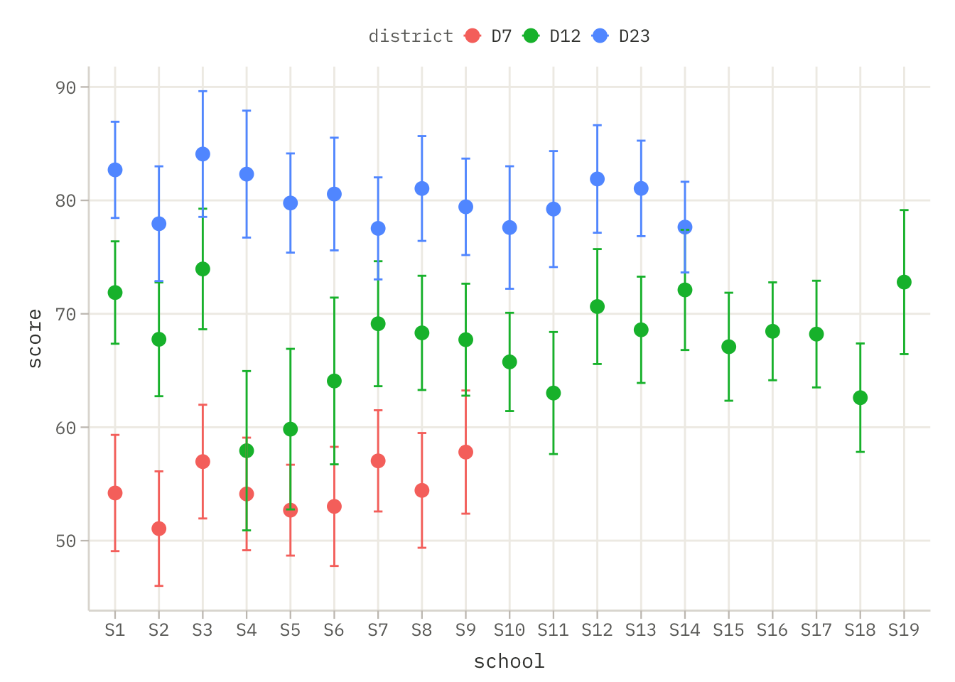
So she plotted every school as its own point, coloured by district, each district’s mean drawn as a horizontal bar behind its schools. Three coloured clouds climbed the chart, red District 7 low, gold District 12 in the middle, blue District 23 on top, each cloud sitting fairly tight around its own bar. Except District 12 was not quite tight. Most of its nineteen schools clustered in the high sixties and low seventies, where a middle-district school ought to be. But one point had fallen out of the cloud entirely. It sat far below the others, below the whole gold band, below even the red District 7 mean, alone in the empty space between the districts.
“That’s Bernat’s school,” Bit said. “School 4.”
“Yes.” She did not have to squint at it. This was not a school a few points under its peers; it was a school that had dropped clean out of its own district’s range and landed beneath a poorer district’s average. In District 12, where scores lived in the high sixties, School 4 was pulling something close to fifty-eight. Two of its neighbours, she noticed, sat lower than the rest of the cloud as well, not as far as School 4, but visibly beneath the gold band: School 5 near sixty, School 6 a little above it. Three schools sagging where sixteen others held level.
She built the model that let each school speak for itself. Districts as the upper factor. Schools nested within districts as the lower one, each school a specific level rather than a draw from some larger pool. The nested structure asked two questions in order. First: do the districts differ? Second, the one that mattered for Bernat: once the district staircase is accounted for, do schools within the same district still differ from each other?
Both terms came back overwhelmingly significant. The district effect was vast, no surprise, the staircase was real. But the school-within-district term was strongly significant too, and District 12 was carrying most of that weight. Schools sharing a district were not interchangeable. Something specific to School 4, and to a lesser degree its two sagging neighbours, was dragging their scores down, over and above the district they belonged to. Bernat’s intuition now had a statistical shape.
But a significant school term only says the schools differ. It does not say why. Beta had proven that School 4 sat apart from its District 12 peers; she had not yet named the reason. If the between-district gradient was wealth, what was the extra thing bending this handful of schools downward, and could it be turned from unexplained school-to-school noise into a variable with a name? Two unused columns still sat in the export. One of them was NutriFirst.
She added it to the model, alongside the observation week, keeping the nested structure underneath. Week did nothing; scores were not drifting over the monitoring period. But NutriFirst did not merely matter. It detonated. After the district staircase had taken its enormous share of the variation, programme membership still explained a further slice so large the F-statistic ran into the hundreds, far past anything chance could manufacture, and it pointed unambiguously downward. Schools on the NutriFirst cartridges scored far below where their district and their peers would otherwise place them.
Bit pulled the enrolment records while she re-read the coefficient. Then he stopped, because the enrolment list matched the plot exactly. School 4 was on NutriFirst. So were School 5 and School 6, the two other schools that had sagged beneath the District 12 band. Every remaining school in District 12 was on the standard municipal supply. The three schools the nested model had flagged were precisely the three schools eating the cartridges. And the batch had a name in the logistics feed: SB-2046-NF-07.
“Three schools on the programme, sixteen not,” Bit said. “That’s why they stand out. They have neighbours to stand out against.”
“Right,” Beta said. “And now look at District 7.” She filtered the enrolment column by district and went still. In District 7, every school read the same value. All nine on NutriFirst. All nine on batch SB-2046-NF-07. “In District 12 the programme reaches three schools out of nineteen, so they drop below the others and the model catches them. In District 7 it reaches everyone. Nine schools, all on the cartridges, all scoring the same low, no school left on normal food to compare against. When everyone eats the same bad food, the data looks perfectly normal. The whole district just sits at the floor and the average calls it poverty.”
She could not prove causation from this alone. She had a nested model that isolated real school-level differences, a programme indicator with a colossal, negative, unmistakable effect, and three District 12 schools that had joined the programme and fallen out of their own district’s range. It was an association, but an association this clean, lined up this precisely with who ate what, was hard to look away from. And it reframed the entire District 7 gradient. What everyone had read as poverty might be, in large part, the cartridges themselves, invisible in District 7 precisely because they covered the whole district evenly, and visible in District 12 only by the accident that most of its schools had been spared them.
She wrote two documents. The first was the statistical report: the nested ANOVA tables, the school-within-district term, the NutriFirst coefficient and its confidence interval, the enrolment records cross-referenced by school and batch number. The second was shorter, addressed to the health office.
NutriFirst cartridges from batch SB-2046-NF-07 are associated with severely lower NutritionScore outcomes, over and above district and school effects. In District 12 the programme reaches only three schools, which fall far below their district baseline. In District 7 the same batch is the primary food supply for every school, where its effect is masked by the absence of any within-district comparison group. We recommend independent biochemical analysis of cartridge protein bioavailability before the next procurement cycle.
Then a note to Bernat, without notation: Your students aren’t tired because they aren’t trying. School 4 is one of only three schools in your district on the NutriFirst cartridges, and it shows in the scores. The data didn’t hide that from you. It only hid it from everyone who read the numbers one district at a time.
Outside, District 12 School 4 was dark. Somewhere in District 7, nine schools were preparing for Monday, every one of them on the same batch, none of them standing out. Same cartridges. Same scores. The same data that looked, in aggregate, perfectly unremarkable, right up until someone refused to stop at the average.
7.2 The Formula: Nested ANOVA
In this chapter, we’ll present an example of two-way analysis of variance in which levels are not crossed as in Section 6.2, but are nested. Crossed means that every combination of levels of both variables can occur in the data. For example, gender and eye color can be variables that can be crossed because both women and men can have blue eyes, so all combinations of eye color and gender could be observed in the dataset. Pairs of variables that are not crossed, but nested, include, for example, country and city. The city effect is nested in the country effect, Warsaw, Wrocław, Poznań, and other Polish cities occur only in Poland (even if cities with these same names also occur in other countries, they are different cities).
Below, we’ll show what matrix \(X\) and vector \(y\) look like in the case of two-way analysis of variance with nested effects, case which is sometimes called hierarchical analysis of variance. As in the previous chapters, our main focus is on statistical tests to verify whether a particular variable is significant or not. In the case of nested variables, this raises the question of at what level of nesting we observe significant differences between objects. Think of examples like:
We analyse variation in exam results on a nationwide scale. One of the considered factors may be the province effect; we can also consider the city or municipality effect. The municipality effect is nested in the province effect. We can additionally consider a variable indicating high school and speak of the high school effect, which is nested in the province effect. We can also consider the class effect; considering all four nested variables simultaneously, we have a four-level hierarchical model.
We analyse a child’s level of mathematical ability, but we also want to take the family effect into account. There are families with several children, and in such cases it is better to consider the individual effect of the child as an effect nested within the parental effect.
7.2.1 The Model
Let’s consider two categorical variables A and B. Assume that variable A can occur at \(k\) different levels, and variable B is nested in A and for the \(i\)-th level of variable A can occur at \(n_i\) levels. The number of groups defined by this pair of variables is \(\sum_{i=1}^k n_i\).
Let \(n_{i,j}\) denote the number of observations measured for the pair of factors \(A=i\) and \(B=j\). Denote by \(y_{ijk}\) the value of the \(k\)-th individual in this group.
where trait \(y\) has a normal distribution with variance \(\sigma^2\) and mean \(\mu_{i,j}\). If \(n_{i,j}\) is the same in each group, we speak of a balanced design; otherwise, an unbalanced design.
Hypotheses posed in two-way hierarchical analysis of variance concern the values of means \(\mu_{i,j}\) or \(\mu_i\). Let’s present these means in Equation 7.1; in each row there may be a different number of means because a different number of levels of variable B may be nested in variable A.
This table of means can be presented in a different parameterization. If we denote by \(\alpha_i\) the additive effect of the first factor and by \(\beta_{i,j}\) the additive effect of the second factor, then we can present the table of means Equation 7.2 in a new parameterization.
To ensure identifiability of parameters in the model, constraints must be added to the new parameters. In line with the previous chapters, the following constraints are adopted:
\(\alpha_i\) is the fixed effect of level \(i\) of factor \(A\) (district),
\(\beta_{j(i)}\) is the fixed effect of school \(j\) nested within district \(i\),
\(\varepsilon_{ijk} \sim \mathcal{N}(0, \sigma^2)\) is the residual error.
The notation \(\beta_{j(i)}\) — read “beta j within i” — indicates that school \(j\) is not an independent factor but is defined only within a specific district. School 4 in District 12 is a different entity from School 4 in District 7, even if they share a label.
Translating the above description into the language of linear models, we’ll consider a linear model of the form:
\[
y = X \beta + \varepsilon,
\]
in which vector \(\beta = (\mu, \alpha_2, \ldots, \alpha_k, \beta_{1,2}, \ldots, \beta_{k,n_k})\), and matrix \(X\) is a matrix of indicators of individual factors. The first column of matrix \(X\) will be filled with ones, the next \(k-1\) columns will encode levels of variable A, and the last \(\sum_{i=1}^k (n_i - 1)\) columns will encode levels of variable \(B\).
For example, assume we have a set of eight observations and three variables: one quantitative \(y\) and two categorical \(x_1\) and \(x_2\). Assume that variable \(x1\) occurs at two levels: C or D, and the number of occurrences of each level is balanced and equals four occurrences. In other words, the variable \(x=c(C, C, C, C, D, D, D, D)\) describes two four-element groups. Assume that variable \(x_2\) is nested in variable \(x_1\) and occurs at levels nested in variable \(x_1\): Q_C, R_C, or Q_D, R_D. The variable is \(x_2=c(Q_C, Q_C, R_C, R_C, Q_D, Q_D, R_D, R_D)\).
The formula y~x1/x2 describes a two-way analysis of variance model in which levels of variable x2 are nested in levels of variable x1. The corresponding matrix notation is as follows:
where \((y_{1,1,1}, y_{1,1,2}, \ldots, y_{2,2,1}, y_{2,2,2})\) is an eight-element vector with measurements of trait \(y\), and \((\varepsilon_{1, 1,1}, \varepsilon_{1, 1,2}, \ldots, \varepsilon_{2,2,1}, \varepsilon_{2,2,2})\) is an eight-element vector corresponding to random disturbance \(\varepsilon \sim \mathcal{N}(0, I_{8\times 8}\sigma^2)\).
7.2.2 It’s all about testing
In two-way hierarchical analysis, we test two types of null hypotheses:
Hypotheses related to main effects of variable \(A\). Does the mean of the response variable differ significantly across the possible values at the level of hierarchy variable \(A\) (similar to one-way ANOVA)?
against hypothesis \(H^{II}_A: \ \exists_{i,j} \ \beta_{i,j} \neq 0\).
7.3 The Terminal: Nest to test
The dataset used in this section comes from the RougeLM package. The nutrition dataset contains weekly NutritionScore measurements from 41 schools across three districts of WaszKrak, with additional variables recording whether the school is enrolled in the NutriFirst programme (nutrifirst) and the observation week (week).
head() confirms the structure: each row is one weekly observation for one school. district and school are the two grouping variables; score is the continuous response; nutrifirst is a logical indicator if the school in question take part in the programme; week is an integer recording the observation week within the monitoring period.
7.3.1 School means by district
Before fitting any model it is important to understand the structure of the grouping variables.
# A tibble: 19 × 4
   school    D7   D12   D23
   <fct>  <dbl> <dbl> <dbl>
 1 S1      54.2  71.9  82.7
 2 S2      51.1  67.8  77.9
 3 S3      57.0  74.0  84.1
 4 S4      54.1  57.9  82.3
 5 S5      52.7  59.8  79.8
 6 S6      53.0  64.1  80.6
 7 S7      57.0  69.1  77.5
 8 S8      54.4  68.3  81.0
 9 S9      57.8  67.7  79.4
10 S10     NA    65.8  77.6
11 S11     NA    63.0  79.2
12 S12     NA    70.6  81.9
13 S13     NA    68.6  81.1
14 S14     NA    72.1  77.6
15 S15     NA    67.1  NA
16 S16     NA    68.5  NA
17 S17     NA    68.2  NA
18 S18     NA    62.6  NA
19 S19     NA    72.8  NA
Table 7.1
group_by(district, school) partitions the data by every district-school combination. summarise(avg_score = mean(score)) then collapses each group to its mean NutritionScore. pivot_wider() reshapes the result so that each district becomes a column — making it easy to compare school means across districts in a single glance.
The resulting table reveals something structurally important: School 1 in District 7 is not the same entity as School 1 in District 12. School labels are only meaningful within a district, they are arbitrary identifiers reused across districts. This rules out a crossed (additive) school effect, where a single school coefficient would represent the same school appearing in multiple districts. The only sensible model is one where school effects are nested within districts: each school is a unique unit belonging to exactly one district, and its effect is estimated relative to the other schools in the same district.
If we were to ignore this and include school as an additive main effect, as if school labels were comparable across districts, the model would attempt to estimate a single coefficient for “School 1” by pooling across all districts, which is statistically and substantively meaningless.
7.3.2 Show me the data
Of course, we’ll start by looking at the data. We’d normally use a box plot, as in the previous chapters, but let’s try something different and look at the means and standard deviations across the schools. To plot these, we need to prepare the following in advance
mean_sd is a user-defined summary function that returns a data frame with three columns: y (the mean), ymin (mean minus one standard deviation), and ymax (mean plus one standard deviation). This specific output format, a data frame with columns named y, ymin, and ymax, is required by geom = "errorbar" inside stat_summary(): ggplot2 looks for exactly these names when drawing the bar extents. The na.rm = TRUE argument ensures that any missing scores are silently excluded before computing the mean and standard deviation.
Figure 7.1: Mean NutritionScore per school with ± one standard deviation error bars. Each point is one school’s mean across all weeks; the error bars show the within-school variability. Points are coloured by district. One school in District 12 sits well below all others in its district and below the District 7 mean — the outlier that the nested model will isolate.
stat_summary() computes a summary statistic from the raw data and plots the result directly, without requiring a separate aggregation step. It appears twice here, performing two different operations on the same underlying data:
The first call uses fun = mean and geom = "point": for each school, it computes the mean of all weekly score values and places a point at that value. fun expects a function that takes a vector and returns a single number.
The second call uses fun.data = mean_sd and geom = "errorbar": for each school, it calls the mean_sd function defined above and uses the returned ymin and ymax values to draw the error bar extents. fun.data expects a function that returns a data frame with columns y, ymin, and ymax — which is why mean_sd was written in exactly that format. width = 0.2 controls the horizontal width of the end-caps on the error bars.
Colour is mapped to district in aes(), so all schools belonging to the same district share a colour, making the between-district pattern immediately visible alongside the within-district school variation.
7.3.3 Model witht nested variables
Let’s fit a model with two nested variables. This will correspond to an \(X\) matrix with three components, as shown in Equation 7.4.
Both lines correspond to the same model, they just use different notations. They are shown together to illustrate two equivalent formula syntaxes for nested effects.
The first form, district + district:school, is explicit: district adds a main effect for district, and district:school adds the interaction term between district and school — which, because school is nested within district rather than crossed with it, is equivalent to a separate school effect estimated within each district.
The second form, district/school, uses the nesting operator /. It expands automatically to district + district:school, producing an identical design matrix. The / notation is preferred in practice because it documents the nesting structure directly in the formula, making the model’s intent clear to anyone reading the code. The second assignment overwrites the first; only model_nut_01 from the / formula is used in subsequent steps.
7.3.4 ANOVA table for the nested model
We now test hypothesis Equation 7.5 and Equation 7.6. As they are nested, we can use the likelihood ratio test.
anova(model_nut_01)
Analysis of Variance Table

Response: score
                  Df Sum Sq Mean Sq  F value    Pr(>F)
district           2 271598  135799 5129.172 < 2.2e-16 ***
district:school   39  29006     744   28.091 < 2.2e-16 ***
Residuals       2714  71855      26
---
Signif. codes:  0 '***' 0.001 '**' 0.01 '*' 0.05 '.' 0.1 ' ' 1
Table 7.2
anova() on the nested model produces a sequential ANOVA table with two rows: one for district and one for district:school. Reading the table:
The district row tests whether the between-district variation in mean NutritionScore is larger than would be expected by chance. A significant F-value here indicates that district-level differences in scores exist, which is unsurprising given the known socioeconomic gradient across WaszKrak districts.
The district:school row tests whether the between-school variation within districts, after accounting for the district main effect, is significant. A significant result here means that schools within the same district differ from one another in ways not explained by which district they belong to. This is the key test for the outlier: if one school in District 12 scores dramatically lower than all other District 12 schools, the school-within-district term will be significant.
7.3.5 Adding nutrifirst and week
The nested school structure accounts for the clustering of observations within schools. Once that structure is in the model, we can test whether additional variables, the NutriFirst programme and the observation week, contribute further.
Analysis of Variance Table

Response: score
                  Df Sum Sq Mean Sq   F value Pr(>F)
district           2 271598  135799 5665.6456 <2e-16 ***
nutrifirst         1  19601   19601  817.7641 <2e-16 ***
week               1     43      43    1.8135 0.1782
district:school   39  16213     416   17.3444 <2e-16 ***
Residuals       2712  65004      24
---
Signif. codes:  0 '***' 0.001 '**' 0.01 '*' 0.05 '.' 0.1 ' ' 1
district/school retains the nested structure established in model_nut_01. The additional terms + nutrifirst + week add the programme indicator and the temporal trend as additive main effects. nutrifirst is a logical or factor variable encoding whether the school receives NutriFirst cartridges; week captures any linear trend in scores over the monitoring period.
anova() now produces four rows: district, district:school, nutrifirst, and week. Each term is tested sequentially, conditional on all terms listed before it. The nutrifirst row answers the primary question: after accounting for district, school-within-district, and the temporal trend, does NutriFirst programme membership explain additional variation in NutritionScore?
7.4 Exercises
7.4.1 Exercise 1: Extracting the NutriFirst effect
Beta has fitted model_nut_02 which includes district, school nested within district, NutriFirst programme membership, and observation week.
(a) Extract the coefficient for nutrifirst from the fitted model using coef(). What does the sign and magnitude of this coefficient tell you about the association between the NutriFirst programme and NutritionScore?
(b) Use confint() to compute a 95% confidence interval for the nutrifirst coefficient. Does the interval contain zero? What does this tell you about the statistical significance of the NutriFirst effect, and how does your answer relate to the p-value in anova(model_nut_02)?
(c) The week coefficient is also present in the model. Using coef(), extract its value and interpret it: how does NutritionScore change on average for each additional week of monitoring, holding all other variables constant?
7.4.2 Exercise 2: Crossed versus nested structure
A student proposes fitting the following model instead of model_nut_01:
model_wrong <-lm(score ~ district + school, data = nutrition)
(a) How many coefficients does model_wrong estimate for the school term? How many coefficients does model_nut_01 (with district/school) estimate for the school-within-district term? Use length(coef()) on both models to check. Explain the difference.
(b) Run head(model.matrix(model_wrong)) and head(model.matrix(model_nut_01)). Compare the two design matrices. What is the key structural difference between how the two models encode the school variable? Which encoding correctly reflects that School 1 in District 7 and School 1 in District 12 are different entities?