It was 2:47 a.m. when Bit stopped typing and looked at the wall, the actual wall, covered in printouts from twelve months of work. MedScore and the partner correlation. CuriosityScore and the four corporations. MobilityScore crossing between junior and mid. NutritionScore and the wrong batch in School 4. EmploymentScore and the slopes that cancelled out. Six cases. Six datasets.
“We’ve been studying the same thing all year,” he said. “Every one of those scores is an input to LifeCalc. It predicts one number for each resident, SocialScore, and that number decides everything else. We’ve been reading its variables one at a time.”
Beta looked at the wall for a long moment. “Then let’s build the whole thing at once, and find out what LifeCalc is really measuring.”
The dataset held five thousand residents. Fifty-one predictors each, every one a Score, the full behavioural and psychometric apparatus the city recorded, and one target column: SocialScore.
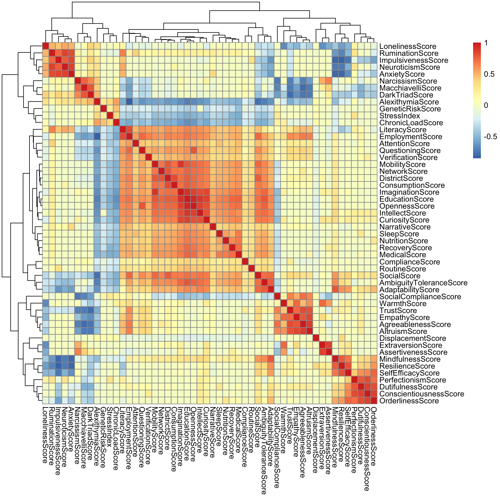
She did what she always did before modelling anything. She looked. Fifty-one predictors do not fit in a scatter plot, so she computed every pairwise correlation, let a clustering algorithm arrange them, and rendered the matrix as a heatmap. It was not fifty-one independent things. Whole blocks glowed the deep red of near-perfect correlation: Education, Network, Mobility, Openness and Intellect fused into one cognitive-social mass; a darker knot of Narcissism, Machiavelli and DarkTriad; an anxiety cluster of Rumination and Neuroticism.
“They all move together,” Bit said. “They’re produced by the same system.”
“Which means we can’t just put all fifty-one in a regression and read the coefficients.” She did it anyway, to show him, then pulled out two: NetworkScore and DistrictScore, which the heatmap showed were almost the same variable. NetworkScore alone against SocialScore was strongly significant. Add DistrictScore and NetworkScore collapsed to nothing. Reverse the order and the verdict flipped: District mattered, Network didn’t.
“Same two variables, opposite answers, depending only on which enters first,” she said. “The model can’t separate them. Ask which one matters and it names a different culprit every time you reshuffle. That’s multicollinearity, and with fifty-one correlated scores it’s everywhere.” The variance inflation factors confirmed it: the correlated predictors were far past the point where any single coefficient could be read on its own.
“So the model’s useless.”
“The coefficients are. Not the model.” Because a model that could predict SocialScore from these scores was not a description of a person. It was a lever, and she wanted to know how short and sharp that lever could be made. She went after it three ways.
An automatic stepwise search pruned the full model under an information criterion, throwing out a dozen redundant scores and keeping a compact core. Then lasso, whose penalty drove coefficients to exactly zero and left them there; she watched variables switch on one by one as the penalty relaxed, and read off the survivors that cross-validation kept. DistrictScore carried the heaviest weight by far, the rest trailing behind it. Then ridge, which shrank every coefficient smoothly toward zero without eliminating any, splitting the credit evenly across each correlated block rather than picking a winner. Different philosophies, same finger: District dominated, and everything else looked like elaboration on where a person started.
“Both point the same way,” Beta said. “But pointing isn’t proof. A coefficient can look big and predict nothing.” So she took every model, full, stepwise, lasso, ridge, and turned them on a thousand residents none had seen, and asked how well each predicted the real SocialScore. The lean models, stepwise and lasso, predicted the unseen lives almost perfectly, explaining nearly all of the out-of-sample variance with error barely above two points on a hundred-point scale. A dozen scores discarded, no accuracy lost. Ridge, keeping everything, did worse.
Bit sat still. “Almost perfect. From a handful of variables.”
“From a handful, led by the one that says which district you were born in.” Beta looked back at the wall, twelve months of cases resolving into a single equation. LifeCalc dressed SocialScore in fifty-one traits, curiosity, empathy, resilience, discipline, as though it were measuring who you had become. Strip the redundancy and something plainer showed through.
“So what do we do with it?” Bit asked.
She didn’t answer right away. The model was sitting there, fitted and validated, and it could be read more than one way. It named the variable that mattered most. It also named the price of dropping each variable that didn’t. Whether that made it a verdict on people or an argument against the system that built it depended entirely on which numbers you pulled out of it next, and how honestly you were willing to read them.
She saved the analysis and opened the model again, the correlation matrix first, so that whatever she concluded, she would not forget that the fifty-one columns had only ever been a few things saying themselves over and over. The rest was in the data. She started to read it.
9.2 The Formula: Multiple Regression, Model Selection, and Regularization
In the previous chapters, we analysed low-dimensional relationships between two, three, or sometimes four variables. There were few variables, but this allowed us to examine carefully which ones should be included in the model and how. How to code a variable, whether to account for interactions, and whether factors overlap or are nested. In the wild, we very often have to deal with many variables, some of which are important and others irrelevant. It is therefore time to look at the tools that will enable us to handle dozens or even more variables.
9.2.1 The Model
In all previous chapters, Beta worked with models containing one or two predictors. The LifeCalc analysis required extending this to the general case. The multiple linear regression model with \(p\) predictors takes the form:
where \({y}\) is the \(n \times 1\) response vector, \({X}\) is the \(n \times
(p+1)\) design matrix, \({\beta}\) is the \((p+1) \times 1\) coefficient vector, and \(\boldsymbol{\varepsilon} \sim \mathcal{N}({0}, \sigma^2 {I})\).
As it was derived in Equation 3.5, the OLS estimator for \(\beta\) is:
assuming that \({X}^T {X}\) is invertible, which fails when predictors are perfectly collinear, and becomes numerically unstable when they are highly correlated.
9.2.2 Multicollinearity and VIF
When predictors are correlated, the Variance Inflation Factor (VIF) measures how much the variance of each coefficient estimate is inflated relative to the case of orthogonal predictors:
\[\text{VIF}_j = \frac{1}{1 - R^2_j} \tag{9.4}\]
where \(R^2_j\) is the coefficient of determination from regressing predictor \(j\) on all other predictors. As rule of thumb, VIF above 10 indicates severe multicollinearity, the coefficient estimate for that variable is unreliable and should not be interpreted independently.
In Beta’s analysis, all six known LifeCalc variables had VIF above 10, because each was partially determined by the same underlying factors (district, prior status) that drove all the others. The system had been designed as a feedback loop; the statistics of that loop showed up as multicollinearity in any model that included multiple variables simultaneously.
9.2.3 Model Selection: AIC and BIC
When building a model, we usually want it to include only relevant variables. Even if we have many variables at our disposal, we do not want to include in the model any unnecessary variables that are unrelated to the response variable. But how do we decide which variables to keep and which to remove? There are many procedures, but some of the most popular involve using the AIC or BIC model selection criteria. From the set of possible models, we select the one that optimises the specified criterion.
Both criteria are based on the likelihood function for a given model (see Equation 3.10) and a penalty for model complexity. For a variable to remain in the model, its contribution to the reduction in the log-likelihood must be greater than the specified complexity penalty.
The Akaike Information Criterion (AIC) for model with \(p\) predictors and corresponding \(\hat \beta_p\) coefficients is defined as:
Both criteria balance fit against complexity, lower values indicate better models. BIC’s stronger penalty for \(k\) means it tends to select sparser models than AIC. In Beta’s analysis, AIC selected approximately eight variables while BIC selected five, both far fewer than the forty-seven available, consistent with a data-generating process driven by a small number of true predictors surrounded by correlated proxies.
9.2.4 Regularization: Ridge Regression
As it was already introduction in Section 3.3.5, ridge regression addresses the problem of high variance of \(\hat \beta\), either due to high \(p\) or high colinearilyt, by adding a penalty on the sum of squared coefficients to the OLS objective:
The regularization parameter \(\lambda \geq 0\) controls the trade-off: \(\lambda = 0\) recovers OLS; as \(\lambda \to \infty\), all coefficients shrink toward zero. Ridge keeps all variables in the model but shrinks their coefficients, useful when all predictors are believed to carry some information.
9.2.5 Regularization: LASSO Regression
As it was already introduction in Section 3.3.6, the Least Absolute Shrinkage and Selection Operator (LASSO) replaces the \(L_2\) penalty with an \(L_1\) value penalty:
where \(\|{\beta}\|_1 = \sum_{j=1}^{p} |\beta_j|\). The \(L_1\) penalty has a geometric property that Ridge lacks: it produces exact zeros for coefficients of unimportant predictors, performing simultaneous estimation and variable selection.
The optimal \(\lambda\) is typically chosen by cross-validation, minimizing out-of-sample prediction error across \(K\) folds. In Beta’s analysis, LASSO with cross-validated \(\lambda\) reduced forty-seven variables to eight, identifying the true predictors from a sea of correlated proxies.
9.3 The Terminal: Multiple Regression in R
The dataset used in this section comes from the RougeLM package. lifecalc contains 5,000 WaszKrak residents scored by the LifeCalc algorithm. The first column, SocialScore, is the outcome variable; the remaining 51 columns are personality and behavioural scores that serve as candidate predictors.
dim() returns the dimensions of the data frame as a two-element vector: number of rows followed by number of columns. Checking dimensions before any analysis is a basic sanity check, it confirms that all expected rows and columns are present and that no silent subsetting has occurred during import. With 51 candidate predictors, this is also a dataset where automatic variable selection will be necessary: fitting all predictors simultaneously produces an over-parameterised model that is difficult to interpret and prone to multicollinearity.
9.3.1 Show me the data
With 51 predictors, inspecting pairwise correlations individually is impractical. A heatmap of the full correlation matrix reveals the block structure at a glance.
Figure 9.1: Heatmap of the pairwise Pearson correlation matrix for all variables in the lifecalc dataset. Rows and columns are reordered by hierarchical clustering so that groups of correlated variables appear as contiguous coloured blocks. Warm colours indicate positive correlations; cool colours indicate negative correlations. Blocks of similarly coloured cells reveal clusters of variables that move together — a visual signal of multicollinearity.
cor(lifecalc) computes the 52 × 52 matrix of pairwise Pearson correlations between all columns, including SocialScore. The result is a symmetric matrix with ones on the diagonal.
pheatmap() from the pheatmap package renders this matrix as a colour-coded heatmap. By default it applies hierarchical clustering to both rows and columns, reordering them so that groups of mutually correlated variables appear adjacent. This clustering is purely visual: it does not affect the correlation values, only their arrangement on the plot. Variables that are strongly positively correlated with each other form warm-coloured blocks; negatively correlated pairs appear in cool colours.
The heatmap answers the diagnostic question before any model is fitted: are there clusters of highly correlated predictors? If yes, including all members of a cluster simultaneously in a regression model will inflate their standard errors and make individual coefficient estimates unreliable, the multicollinearity problem that motivates variable selection and regularisation.
9.3.2 Multicollinearity: an ilustrative example
The heatmap in Figure 9.1 shows that NetworkScore and DistrictScore are strongly correlated. The following sequence of models demonstrates the practical consequence of this correlation for variable selection.
model_NetwDist <-lm(SocialScore ~ NetworkScore + DistrictScore,data = lifecalc_small)model_Netw <-lm(SocialScore ~ NetworkScore, data = lifecalc_small)model_Dist <-lm(SocialScore ~ DistrictScore, data = lifecalc_small)model_0 <-lm(SocialScore ~1, data = lifecalc_small)
Four models are fitted on the same data. model_0 is the intercept-only model, it predicts SocialScore as the sample mean for every observation and serves as the null baseline. model_Netw and model_Dist each include one predictor; model_NetwDist includes both simultaneously.
Let’s compare the results of two analyses of variance (ANOVA) for these three variables, changing only the order in which the variables are included in the model.
anova(model_0, model_Netw, model_NetwDist)
Analysis of Variance Table

Model 1: SocialScore ~ 1
Model 2: SocialScore ~ NetworkScore
Model 3: SocialScore ~ NetworkScore + DistrictScore
  Res.Df     RSS Df Sum of Sq      F    Pr(>F)
1     49 27899.4
2     48 14019.9  1   13879.5 70.237 6.925e-11 ***
3     47  9287.7  1    4732.1 23.947 1.205e-05 ***
---
Signif. codes:  0 '***' 0.001 '**' 0.01 '*' 0.05 '.' 0.1 ' ' 1
Table 9.1: Sequential ANOVA adding NetworkScore first, then DistrictScore. The first row tests whether NetworkScore improves fit over the null model; the second tests whether DistrictScore adds further improvement after NetworkScore is already in the model.
anova(model_0, model_Dist, model_NetwDist)
Analysis of Variance Table

Model 1: SocialScore ~ 1
Model 2: SocialScore ~ DistrictScore
Model 3: SocialScore ~ NetworkScore + DistrictScore
  Res.Df     RSS Df Sum of Sq       F   Pr(>F)
1     49 27899.4
2     48  9641.1  1   18258.3 92.3948 1.13e-12 ***
3     47  9287.7  1     353.4  1.7884   0.1876
---
Signif. codes:  0 '***' 0.001 '**' 0.01 '*' 0.05 '.' 0.1 ' ' 1
Table 9.2: Sequential ANOVA adding DistrictScore first, then NetworkScore. The order is reversed: DistrictScore is tested against the null, then NetworkScore is tested conditional on DistrictScore already being present.
anova() with three model arguments performs two sequential likelihood ratio tests. Each test compares adjacent models in the sequence: the first test asks whether moving from model_0 to the one-predictor model significantly reduces the residual sum of squares; the second asks whether adding the remaining predictor further reduces it.
Comparing the two tables reveals the asymmetry introduced by multicollinearity. In the first sequence, NetworkScore alone is highly significant, it captures substantial variance in SocialScore. But when DistrictScore is already in the model, adding NetworkScore is no longer significant: the variance that NetworkScore would have explained has already been absorbed by DistrictScore. In the second sequence the pattern reverses: DistrictScore alone is significant, and NetworkScore conditional on DistrictScore is not.
This is the defining feature of multicollinearity: neither variable is unimportant, but because they carry largely the same information, the model cannot distinguish their individual contributions once either one is present. The order in which predictors enter the sequential ANOVA determines which one appears significant, a consequence of the sequential (Type I) sum of squares used by anova().
We must therefore be careful when testing and removing variables from a model in which the variables are correlated.
9.3.3 The full model
Before we move on to variable reduction and regularisation, let’s start with the full model, which includes all 51 variables, regardless of their internal correlation.
model_Full <-lm(SocialScore ~ ., data = lifecalc)
lm(SocialScore ~ ., data = lifecalc) fits the full model with all predictors. The . on the right-hand side of the formula is a shorthand meaning “all other columns in the data frame”.
9.3.4 Automatic variable selection with step()
With 51 candidate predictors, manual model variable selection is not feasible. The step() function automates variable selection by iteratively adding or removing one predictor at a time, accepting changes that improve a specified information criterion (by default AIC, but we will force BIC with \(k=log(n)\) penalty).
9.3.4.1 Backward predictor elimination
One strategy to automate predictor elimination is to start from the full model and applies backward elimination: at each step it considers dropping each predictor currently in the model and retains the change if it improves the criterion. This can be done with the step() function.
model_Full <-lm(SocialScore ~ ., data = lifecalc)model_step1 <-step(model_Full, k =log(5000), trace =0)
The argument k controls the penalty per parameter in the information criterion: k = 2 gives AIC; k = log(n) gives BIC, which applies a stronger penalty for model complexity and typically selects fewer predictors. Here k = log(5000) uses BIC with the sample size of the lifecalc dataset. trace = 0 suppresses the step-by-step output; setting trace = 1 would print a summary of each step to the console.
9.3.4.2 Forward predictor selection
Another strategy to automate predictor selection is to start from the empty model and applies forward selection: at each step it considers adding one predictor to the model. This also can be done with the step() function.
step(,direction = "forward") applies forward selection starting from the intercept-only model. Three components differ from model_step1:
lm(SocialScore ~ 1, data = lifecalc) is the starting model, the null model with no predictors, equivalent to model_0 above.
scope = list(upper = formula_Full, lower = ~ 1) defines the search space. upper is the most complex model allowed (all predictors); lower is the simplest model allowed (intercept only). At each step, step() may only add predictors that are in upper but not yet in the current model. formula_Full is constructed programmatically: colnames(lifecalc)[-1] extracts all column names except SocialScore; paste(..., collapse = "+") joins them with + separators; as.formula() converts the resulting string into a formula object that lm() can use.
direction = "forward" restricts the search to additions only, predictors are never removed once added. This is the key difference from backward elimination. Forward and backward selection explore different paths through the space of possible models and often arrive at different final models, because the optimality of adding a predictor depends on which other predictors are already present.
Let’s check which variables were removed from the model model_step1 and model_step2.
It looks like both approaches remove 12 predictors from the model but different ones. As far as the number of variables in the model is concerned, the two approaches appear similar, but we will check later whether these models differ in terms of predictive performance.
9.3.5 LASSO variable selection
A popular alternative to manually selecting variables is to use the LASSO procedure. It imposes a penalty on the magnitude of the coefficients, but an additional effect is that it automatically removes certain variables from the model.
We will illustrate this using the glmnet() function; however, this requires the data to be a numeric matrix rather than a data frame.
lifecalc[, -1] drops the first column (SocialScore) and retains all 51 predictors; as.matrix() converts the result to the required format. y is the response vector extracted separately.
glmnet standardises the columns of X internally by default (standardize = TRUE), so variables measured on different scales are placed on a common footing before the penalty is applied.
model_lasso_1 <-glmnet(X, y, alpha =1)
The glmnet() function allows you to estimate coefficients using a broad family of models, known as the elastic net regularization, which is parameterised by the alpha coefficient. If you set alpha to 1, you will obtain the LASSO estimation method.
glmnet(X, y, alpha = 1) fits the LASSO model across an automatically chosen grid of penalty values \(\lambda\). The function does not fit a single model but an entire regularisation path: one set of coefficient estimates for each value of \(\lambda\), from \(\lambda_{\max}\) (large enough that all coefficients are zero) down to a small \(\lambda\) close to the OLS solution. The result is a glmnet object containing the estimates of coefficients for all selected values of \(\lambda\).
Usually, to select the best \(\lambda\), a procedure called cross-validation is used. The quality of the prediction results obtained for a given \(\lambda\) is assessed, and the \(\lambda\) with the lowest prediction error is selected.
set.seed(2047)model_lasso_cv <-cv.glmnet(X, y, alpha =1, nfolds =10)
9.3.5.1 Selection of \(\lambda\)
cv.glmnet() selects the optimal \(\lambda\) by 10-fold cross- validation. For each value of \(\lambda\) on the path, the dataset is split into 10 folds: the model is trained on 9 folds and evaluated on the held-out fold, repeating for all 10 rotations. The mean squared error is averaged across folds and plotted against \(\log(\lambda)\). set.seed(2047) ensures that the fold assignment is reproducible.
model_lasso_cv$lambda.1se
[1] 0.01127204
model_lasso_cv$lambda.min
[1] 0.004445925
The cross-validation result provides two reference values:
model_lasso_cv$lambda.min, the \(\lambda\) that minimises the mean cross-validated error,
model_lasso_cv$lambda.1se, the largest \(\lambda\) whose error is within one standard error of the minimum, corresponding to the most parsimonious model that is not significantly worse than the best.
lasso_coef <-coef(model_lasso_cv, s ="lambda.min")head(lasso_coef)
6 x 1 sparse Matrix of class "dgCMatrix"
                  lambda.min
(Intercept)      45.08710146
EducationScore    0.00511494
EmploymentScore  -0.12388883
DistrictScore     0.38137653
LiteracyScore    -0.22357420
QuestioningScore  0.06465224
Table 9.3
coef(model_lasso_cv, s = "lambda.min") extracts the coefficient vector at the optimal \(\lambda\). The result is a sparse matrix with one row per predictor plus the intercept; variables whose coefficient is exactly zero have been eliminated by the LASSO penalty.
9.3.6 The LASSO regularisation path
The glmnet function estimates the \(\beta\) coefficients across the entire range of \(\lambda\) values. We can extract all these partial estimates from the model and plot them as functions of the \(\lambda\) parameters.
coef(model_lasso_1) returns a matrix with one row per predictor and one column per \(\lambda\) value on the path. Transposing with t() and converting with as.matrix() produces a matrix where rows are \(\lambda\) values and columns are predictors, making it easier to work with in a tidy pipeline. The intercept column is dropped with [, -1] because it is not part of the regularised coefficient path.
mutate(log_lambda = log(lasso_lambdas)) adds a column for the log-transformed \(\lambda\) values. Plotting on the log scale spreads the path evenly across the x-axis, on the raw scale, the values cluster near zero where the path is most interesting.
pivot_longer() reshapes the wide matrix (one column per variable) into a long data frame (one row per variable-\(\lambda\) combination), which is the format that ggplot2 requires for plotting multiple lines.
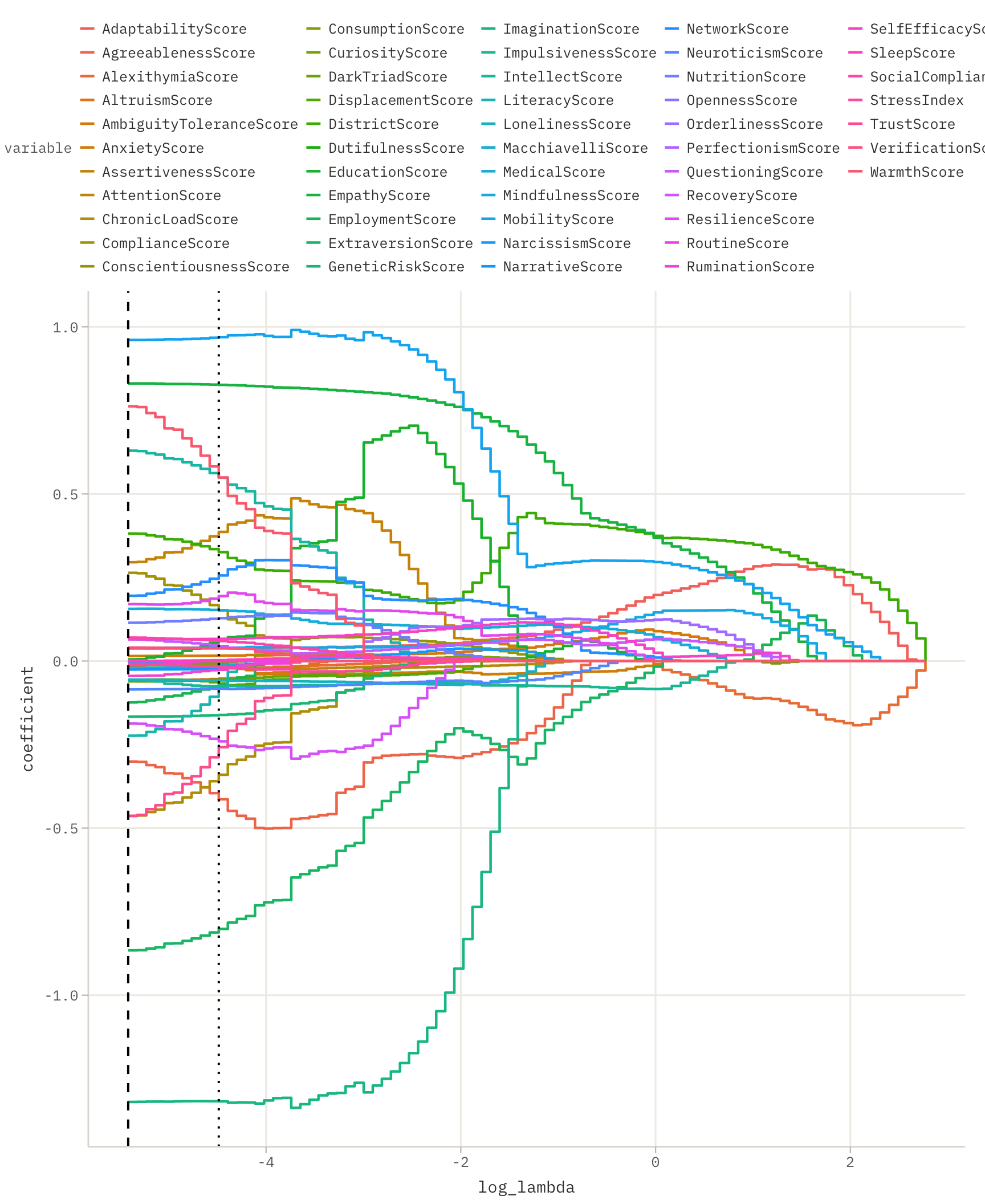
The regularisation path plot is the primary diagnostic for LASSO variable selection. Reading it from left to right traces what happens as the penalty is relaxed: at the leftmost point all coefficients are zero; as \(\lambda\) decreases, the first variable enters the model (its line leaves zero), then the second, and so on. Variables that enter at large \(\lambda\) values have the strongest marginal relationship with SocialScore after accounting for the variables already selected. Variables that never leave zero across the entire path shown are excluded at every penalty level and carry no predictive information beyond what the selected variables already provide.
Figure 9.2: LASSO regularisation path for all 52 predictors of SocialScore. Each coloured line traces the estimated coefficient of one variable as the penalty lambda decreases from left (maximum regularisation, all coefficients zero) to right (minimum regularisation, close to OLS). Variables whose lines reach zero and remain there are eliminated by LASSO. The dashed vertical line marks lambda.min; the dotted line marks lambda.1se.
The two vertical reference lines divide the path into three regions. To the left of lambda.1se the model is parsimonious, only the most important variables have non-zero coefficients, and the model is within one cross-validation standard error of optimal. Between the two lines the model adds more predictors at a cost of slightly higher variance but lower bias. To the right of lambda.min the model approaches OLS and the regularization benefit diminishes.
9.3.6.1 Number of non-zero coefficients as a function of lambda
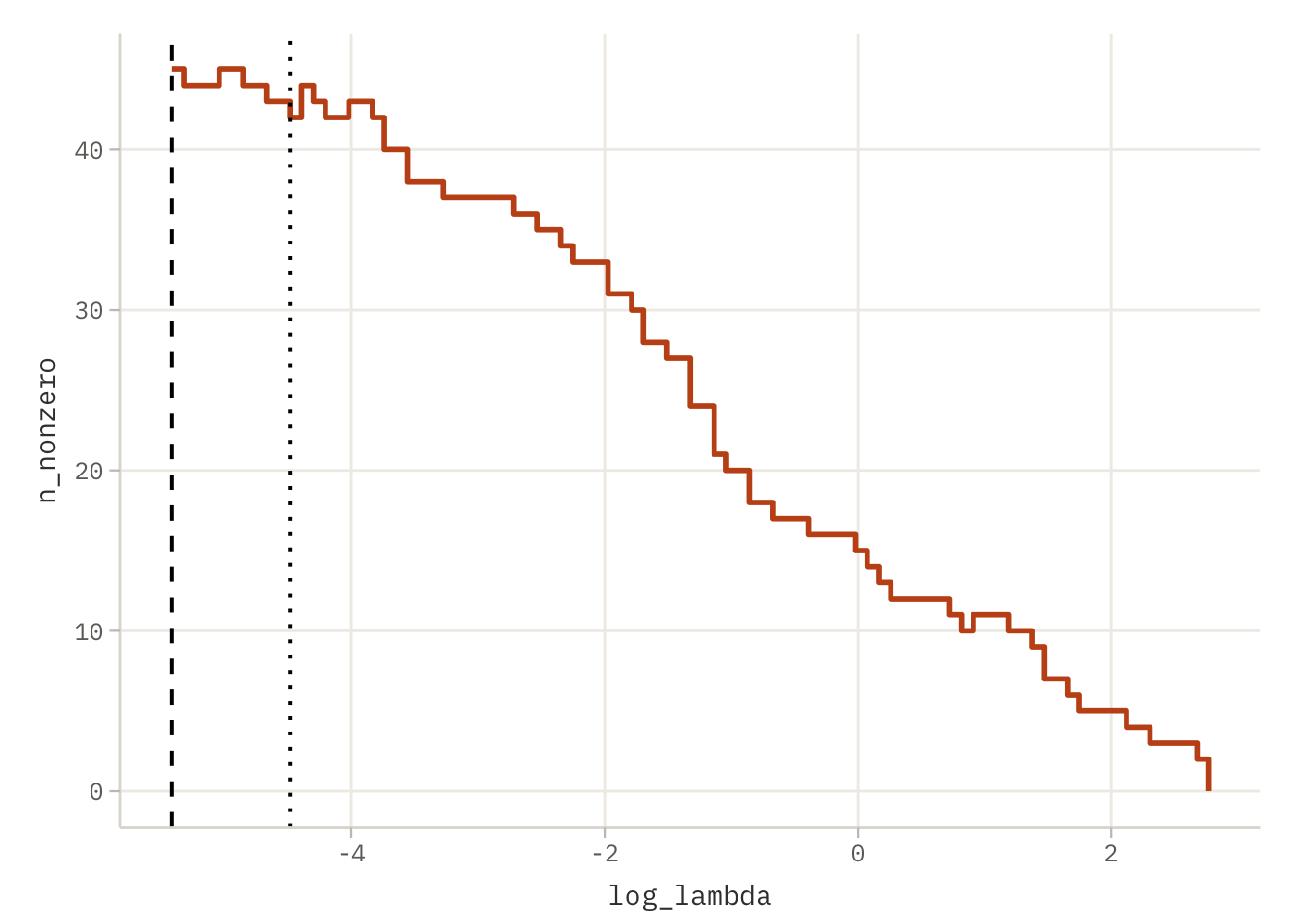
The regularisation path plot shows which variables enter the model as \(\lambda\) changes. A complementary view shows how many variables are selected, a single number that summarises the sparsity of the model at each penalty level.
model_lasso_1$lambda is the vector of \(\lambda\) values at which glmnet evaluated the regularisation path, the same values used for the x-axis of the path plot above. model_lasso_1$df is a vector of the same length, recording the number of non-zero coefficients (degrees of freedom) in the fitted model at each corresponding \(\lambda\).
Figure 9.3: Number of non-zero LASSO coefficients as a function of log(lambda). As the penalty decreases from left to right, more variables enter the model one by one. The step-function shape is characteristic of LASSO: variables are added discretely, not gradually. The dashed vertical line marks lambda.min; the dotted line marks lambda.1se. Reading the y-value at each reference line gives the number of predictors selected by the corresponding criterion.
The two geom_vline() calls add the same reference lines as in the path plot. Reading the y-coordinate at each vertical line gives the model size selected by the corresponding criterion: the y-value at lambda.min is the number of predictors in the cross-validation- optimal model; the y-value at lambda.1se is the number of predictors in the most parsimonious model within one standard error of optimal.
Figure 9.2 and Figure 9.3 answer complementary questions. The path plot identifies which variables are selected and how their coefficients evolve; the count plot shows how many are selected at each penalty level and makes the trade-off between model complexity and regularisation immediately readable.
9.3.7 Ridge regression
Where LASSO sets coefficients to exactly zero and thereby performs variable selection, ridge regression takes a different path: it retains all predictors but shrinks their coefficients continuously toward zero. The amount of shrinkage is again controlled by a penalty parameter \(\lambda\).
We will use glmnet() function again, this time setting alpha = 0 forces ridge regression.
model_ridge_1 <-glmnet(X, y, alpha =0)
glmnet(X, y, alpha = 0) fits the ridge model across the same automatically chosen grid of \(\lambda\) values as the LASSO call above. As with LASSO, the result is a full regularisation path, one set of coefficient estimates per \(\lambda\) is stored in a glmnet object.
set.seed(2047)model_ridge_cv <-cv.glmnet(X, y, alpha =0, nfolds =10)
9.3.7.1 Selection of \(\lambda\)
cv.glmnet() with alpha = 0 performs 10-fold cross-validation for the ridge path, selecting lambda.min and lambda.1se by the same procedure used for LASSO. The set.seed(2047) call ensures that the fold partition is identical to the one used in the LASSO cross-validation, making the two CV error curves directly comparable on the same folds.
model_ridge_cv$lambda.min
[1] 1.597783
The optimal \(\lambda\) values for ridge are typically much larger than those for LASSO.
ridge_coef <-coef(model_ridge_cv, s ="lambda.min")head(ridge_coef)
6 x 1 sparse Matrix of class "dgCMatrix"
                    lambda.min
(Intercept)       2.1431899753
EducationScore    0.0782119614
EmploymentScore   0.0007544501
DistrictScore     0.3151715939
LiteracyScore    -0.0044121757
QuestioningScore  0.1398333910
Table 9.4
coef(model_ridge_cv, s = "lambda.min") extracts the coefficient vector at the cross-validation-optimal \(\lambda\).
9.3.8 The ridge regularisation path
As with the LASSO method, here too we have an estimate of the \(\beta\) coefficients for the entire range of \(\lambda\) values. This allows us to plot their estimates as a function of the \(\lambda\) parameter.
The calculations set out below are similar to those described in Section 9.3.6.
The ridge path is extracted and reshaped by exactly the same pipeline used for LASSO. coef(model_ridge_1) returns a matrix of coefficients at each \(\lambda\); t() transposes it so that rows correspond to \(\lambda\) values; [, -1] drops the intercept; pivot_longer() converts the wide matrix to the long format required by ggplot2.
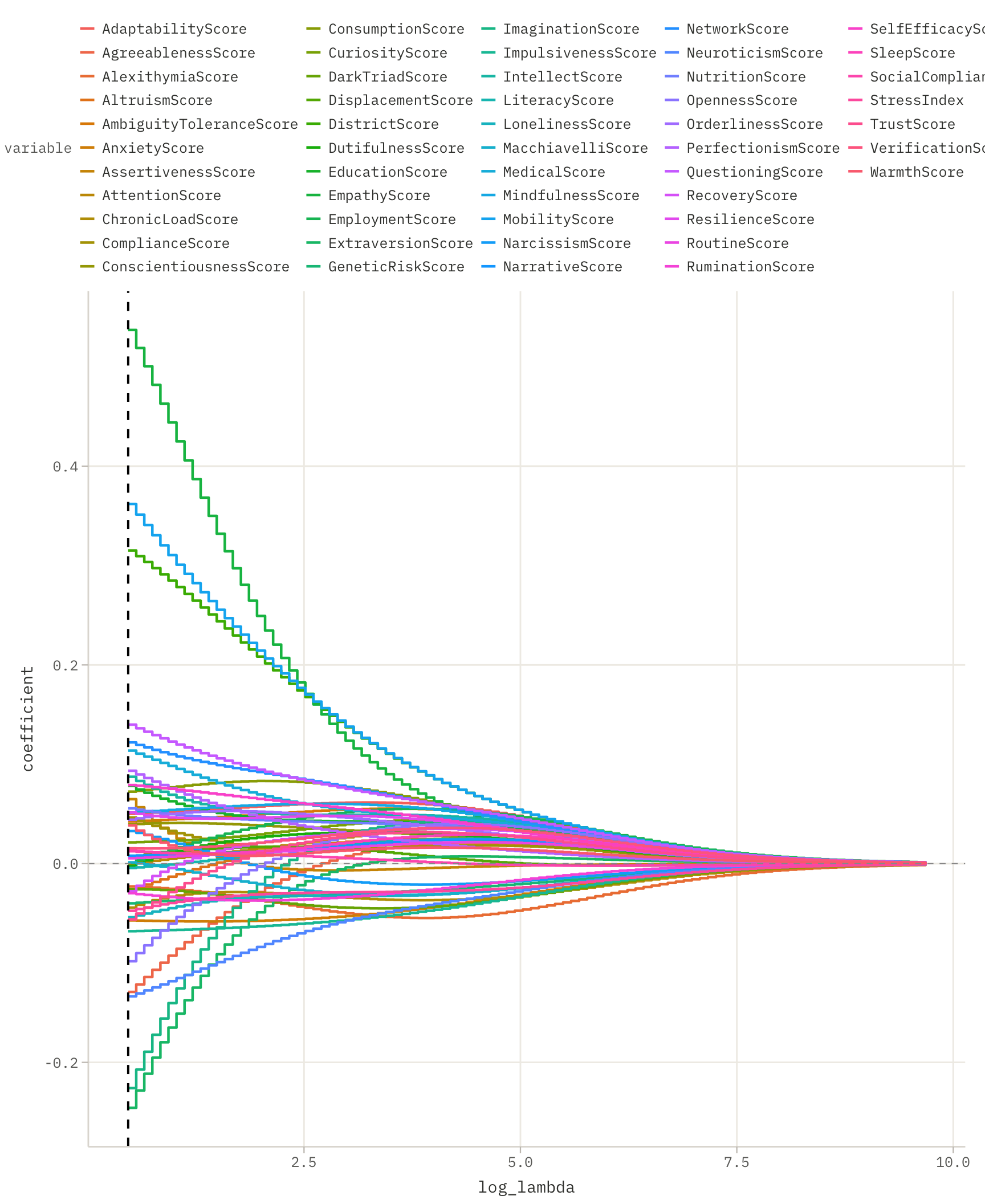
Figure 9.4: Ridge regularisation path for all 52 predictors of SocialScore. Unlike the LASSO path, no line ever reaches zero: all coefficients shrink continuously toward zero as lambda increases, but none is eliminated. At the far right, all lines converge on zero asymptotically. The dashed vertical line marks lambda.min; the dotted line marks lambda.1se.
The ridge path has a distinctly different shape from the LASSO path. In the LASSO plot, lines drop abruptly to zero and stay there producing the characteristic kink at each variable’s entry point. In the ridge plot, every line is smooth and continuous, curving asymptotically toward zero from the right as \(\lambda\) increases.
9.3.9 Predictive performance
In this chapter, we have fitted a number of models predicting SocialScore. Which one should we choose? There may be many criteria, but we will use the model’s predictive performance.
Comparing models on the data used to fit them is misleading. A fair comparison requires new observations that were not seen during estimation. The lifecalc_future dataset provides 1,000 such new observations, a held-out sample from the same WaszKrak population recorded after the training period.
dim(lifecalc_future)
[1] 1000 52
For these new observations the outcome SocialScore is known for every row, so we can compare each model’s predictions against the ground truth and quantify how much of the out-of-sample variance each model explains.
predict() is a generic function that dispatches to the appropriate method depending on the class of its first argument. For lm objects it calls predict.lm() and requires a newdata argument — a data frame with the same column names as the training data; the function locates the predictor columns by name. For cv.glmnet objects it calls predict.cv.glmnet() and requires newx, a numeric matrix with columns in the same order as the training matrix X; the s argument selects which \(\lambda\) to use for prediction. The two interfaces differ because lm and glmnet store their models differently internally.
Table 9.5: Out-of-sample predictive performance on lifecalc_future (n = 1,000) for all models fitted in this chapter. RMSE is the root mean squared error in SocialScore units; MAE is the mean absolute error; R² is the proportion of out-of-sample variance explained. Lower RMSE and MAE and higher R² indicate better predictive accuracy.
Three helper functions — rmse(), mae(), and r2() — compute the three standard metrics for predictive accuracy.
In our case, the stepwise forward (BIC) model offers the best predictive performance. For different datasets, other procedures may prove to be more effective. It is standard practice to calculate several candidate models and compare their performance on new data.
9.4 Exercises
To be continued…
9.4.1 Exercise 1: Multicollinearity in practice
The chapter showed that NetworkScore and DistrictScore are strongly correlated, and that their individual significance depends on the order in which they enter the model.
(a) Run the two sequential ANOVA comparisons from the chapter:
For each sequence, report the p-value for the second term (the one added conditional on the first). In which sequence is NetworkScore significant, and in which is it not? Explain in one sentence why the two results are not contradictory.
(b) Compute the Variance Inflation Factor for NetworkScore in the model model_NetwDist using the car package:
library(car)vif(model_NetwDist)
The VIF for predictor \(j\) is defined as \(1 / (1 - R^2_j)\), where \(R^2_j\) is the \(R^2\) from regressing predictor \(j\) on all other predictors. Verify this formula manually by fitting lm(NetworkScore ~ DistrictScore, data = lifecalc_small) and computing \(1 / (1 - R^2)\) from its summary. Does the result match vif(model_NetwDist)?
(c) The chapter states that a VIF above 10 indicates severe multicollinearity. Compute VIF for all predictors in the full model model_Full and count how many exceed 10. What does this imply for interpreting individual coefficients in the full OLS model?
9.4.2 Exercise 2: Stepwise selection and its limitations
(a) The chapter fitted model_step1 (backward BIC) and model_step2 (forward BIC) and found that both removed 12 predictors but different ones. Run:
List the predictors that appear in model_step1 but not model_step2, and vice versa. For at least one discrepant predictor, look up its correlation with DistrictScore in pairwise_cor and suggest why the two procedures disagreed on it.
(b) Rerun backward selection with k = 2 (AIC) instead of k = log(5000) (BIC):
model_aic <-step(model_Full, k =2, trace =0)length(coef(model_aic))length(coef(model_step1))
Which criterion selects more predictors? Is this consistent with the theoretical properties of AIC and BIC described in the chapter?
(c) Stepwise selection is a greedy algorithm, it makes locally optimal decisions at each step without reconsidering earlier choices. Describe one scenario, using the lifecalc variable names, where greedy backward elimination could discard a predictor that would be useful in combination with a predictor added later. Why does this not happen with LASSO?
9.4.3 Exercise 3: LASSO path and variable entry order
(a) From the LASSO regularisation path plot, identify the first variable to enter the model as \(\lambda\) decreases from \(\lambda_{\max}\). This is the single predictor with the strongest marginal association with SocialScore. Verify by running a simple linear regression lm(SocialScore ~ X[, "variable_name"], data = lifecalc) and checking whether it has the highest \(R^2\) among all single-predictor models.
(b) Read off the number of non-zero coefficients at lambda.min and lambda.1se from the count plot. How many predictors are selected by each criterion? By what factor does the model size change between the two reference points?
(c) Extract the LASSO coefficients at lambda.1se and compare them to the coefficients at lambda.min:
coef_min <-coef(model_lasso_cv, s ="lambda.min")coef_1se <-coef(model_lasso_cv, s ="lambda.1se")
For the predictors selected at both penalty levels, do the coefficients at lambda.1se have the same sign as those at lambda.min? Are they larger or smaller in absolute value, and why?
9.4.4 Exercise 4: LASSO versus Ridge: what each method retains
(a) Count the number of non-zero coefficients in ridge_coef at lambda.min. Compare to the count for lasso_coef at the same reference point. Why does Ridge always retain all predictors while LASSO does not, even at identical penalty strength?
(b) Build a side-by-side comparison table of OLS, LASSO, and Ridge coefficients for the five predictors with the largest absolute OLS coefficient:
For which predictors does LASSO shrink the coefficient more aggressively than Ridge? Is this consistent with the geometry of the two penalties described in the chapter?
9.4.5 Exercise 5: Predictive performance and overfitting
(a) Compute the in-sample\(R^2\) for model_Full using summary(model_Full)$r.squared. Then compute the out-of-sample\(R^2\) for pred_full on lifecalc_future using the r2() function from the chapter. How large is the drop between in-sample and out-of-sample \(R^2\)? What does this gap indicate about the full OLS model?
(b) Compare the out-of-sample RMSE of model_Full, model_step1, and model_lasso_cv at lambda.min. Rank the three models from best to worst predictive performance. Does the ranking match your expectation based on the number of predictors each model uses?
(c) LASSO at lambda.1se is typically more parsimonious than at lambda.min, it uses fewer predictors. Using the perf_df table from the chapter, determine whether the stricter penalty at lambda.1se improves or degrades predictive performance relative to lambda.min. Explain the result in terms of the bias-variance trade-off: what does choosing lambda.1se buy, and at what cost?
(d) Beta argues that the best model is not necessarily the one with the lowest RMSE on lifecalc_future, but the one whose selected variables are most interpretable in the context of the LifeCalc investigation. Given the variable names in the lifecalc dataset and the known structure of the data-generating process, which model would you present to the WaszKrak civil rights tribunal, and why?