The press release arrived on Beta’s feed at 7am, pushed by QuantumCorp’s PR algorithm with a confidence score of 94.7%.
“Second Chance: Transforming Lives in Districts 7 and 11. After six months, participants show a mean EmploymentScore gain of 18.4 points. QuantumCorp’s commitment to algorithmic equity delivers measurable results.”
It took three days to find the data. The full participant records weren’t public, but the individual EmploymentScores were technically accessible through the city’s open data portal, cross-referenced with program enrollment flags. Someone at QuantumCorp had forgotten to restrict the join key. Eight hundred and twelve participants, three tracks, EducationScore at enrollment, EmploymentScore before and after, clean, complete, suspiciously well-formatted.
Beta reproduced the headline exactly. But when she regressed the outcome on education alone, the line came out nearly flat: education was not a significant predictor. The program, the summary concluded, worked equally well regardless of what you brought into it. She sat with that. A flat line means one of two things: either education truly does not matter, or it matters in ways that cancel.
The nudge came from Marek Kowalski. The man with the broken elevator, the father whose daughter had been approved for mobility reclassification while he had not. He had kept her encrypted address, and six months later he used it. He knew six people in the two District 7 programs: Track A, entrepreneurship, and Track B, corporate placement. In Track A the men were doing better than before and the women worse. In Track B the pattern reversed. Six people, he admitted, was not a sample. But it told Beta exactly which variables to condition on. If education helped men and hurt women, and if that reversed between tracks, then averaging over gender and track would wash the whole thing out, four opposing slopes summing to nothing, a flat line built from steep ones.
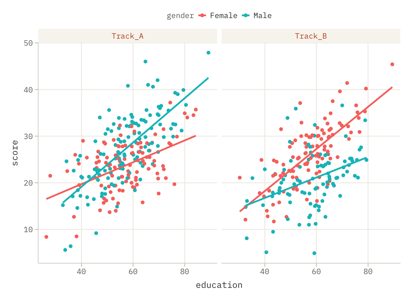
She dropped the third track, simplified gender to two levels, and was left with four hundred and thirty-one participants. Then she plotted EmploymentScore against EducationScore, colored by gender, faceted by track, and the lines crossed. Not with the ambiguity of noise, but cleanly, in both panels, in opposite directions. In Track A, men with more education ended higher and women with more education ended lower. In Track B, the mirror image.
The mechanism, once she traced it, was almost elegant. Track A routed participants through a vendor-registration AI that assessed business viability. It had been trained on fourteen years of small-business outcomes in Districts 7, 11, and 12, years in which surviving businesses were disproportionately founded by men with credentials, not because women ran worse businesses but because educated women in District 7 had historically been channeled into care, tutoring, and community services: sectors the city’s infrastructure classified as low-priority. So when an educated woman entered Track A and chose the sector she was trained for, the viability model read that sector and assigned her a low survival probability, which meant a smaller seed allocation, a lower vendor tier, less visibility in automated procurement. The more education she had, the more confidently she chose the field that the algorithm was calibrated to starve. For men, education opened the sectors the model recognized as high-survival, and the same logic rewarded them.
Track B inverted it. Its placement algorithm, trained on hiring and retention records, read educated women into “high-stability” coordination and compliance roles, stable in the data because women had historically had nowhere else to go, while classifying educated men as overqualified and redirecting them toward higher-turnover technical posts. Neither track was written to discriminate. Both discriminated perfectly.
Beta now had the picture but not the test; a plot suggests where a model decides. The question was not whether education raised EmploymentScore; the flat line had already answered that, misleadingly. The real question had three variables tangled together at once.
“So what do you actually fit?” Bit asked.
“Whether the effect of education depends on gender,” Beta said, “and whether that dependence itself changes between the two tracks.” Within each panel the two gender lines had different slopes, a gender effect on the education slope. But the pattern of that difference flipped between Track A and Track B, and that flip, the difference-in-the-difference, was something no two-variable model could hold. “I need education, gender, and track in the same model, interacting all at once.”
“And if you leave one of them out?”
“You get the press release. A flat line. Two real effects, equal and opposite, adding up to silence.”
She named the dataset employment and reached for the first model.
8.2 The Formula: ANCOVA
In the case of simple regression, we examined relationships between a pair of quantitative variables. In analysis of covariance, we examine the relationship between a pair of quantitative variables in groups described by one or more categorical variables.
8.2.1 The Model
Let’s consider a categorical variable A occurring at \(k\) different levels and quantitative variables \(y\) and \(x\).
The analysis of covariance model is as follows:
\[
y_{j} \sim \mathcal{N}(\gamma_{0,i} + \gamma_{1,i}x_j, \sigma^2), \quad 1 \leq i \leq k, \quad 1 \leq j \leq n,
\]
where trait \(y|A=i\) has a normal distribution with variance \(\sigma^2\) and mean \(\gamma_{0} + \gamma_{1}x\). This corresponds to a simple regression model performed separately for each level of categorical variable \(A\).
Hypotheses posed in analysis of covariance concern parameters \(\gamma_{0,i}\) and \(\gamma_{1,i}\). To better present them, let’s introduce a different parameterization:
Translating the above description into the language of linear models, we’ll consider a linear model of the form:
\[
y = X \beta + \varepsilon,
\]
in which vector \(\beta = (\beta_0, \beta_{0,2}, \ldots, \beta_{0,k}, \beta_{1}, \beta_{1,2}, \ldots, \beta_{1,k})\), and matrix \(X\) is a matrix consisting of four parts. The first two correspond to matrix \(X\) from one-way analysis of variance, the third part corresponds to a column from linear regression, and the fourth part is the product of each pair of columns from the second and third parts (not matrix products but element-wise).
For example, assume we have a set of nine observations and three variables: two quantitative \(y\) and \(x_2\), and one categorical \(x_1\). Assume that variable \(x_1\) occurs at three levels: A, B, or C, and the number of occurrences of each level is balanced and equals three occurrences. In other words, the variable \(x=c(A, A, A, B, B, B, C, C, C)\) describes three three-element groups.
The formula y~x2*x1 describes an analysis of covariance model; the corresponding matrix notation is as follows:
where \((y_{1}, y_{2}, \ldots, y_{9})\) is a nine-element vector with measurements of target variable \(y\), \((x_{1}, x_{2}, \ldots, x_{9})\) is a nine-element vector with measurements of predictor variable \(x\), and \((\varepsilon_{1}, \varepsilon_{2}, \ldots, \varepsilon_{9})\) is a nine-element vector corresponding to random disturbance \(\varepsilon \sim \mathcal{N}(0, \sigma^2 I_{9\times 9})\).
8.2.2 It’s all about testing
Using this parameterization, we can present three different null hypothesesp in analysis of covariance:
Hypotheses related to intercept effects across values of \(A\). Are all intercept levels equal?
against hypothesis \(H^{III}_A: \ \exists_{i} \ \beta_{1,i} \neq 0\).
8.2.3 The Three-Way ANCOVA Model
Beta’s analysis extended the standard ANCOVA framework to accommodate a finding that required all three predictors simultaneously: EducationScore, gender, and program track interacted to produce outcomes that no two-way model could have revealed.
where \(y_i\) is EmploymentScore after program, \(x_i\) is EducationScore at enrollment (the covariate), \(\alpha_j\) is the fixed effect of gender \(j\), \(\gamma_k\) is the fixed effect of program track \(k\), and the remaining terms capture all two-way and three-way interactions between the covariate and the categorical factors.
The three-way interaction term \((\beta\alpha\gamma)_{1jk}\) is the critical one. It captures the degree to which the slope of EducationScore differs by gender, and whether that difference itself differs between tracks. A significant three-way interaction means that the covariate slope is not just different between genders, it is differently different depending on which track you examine.
8.3 The Terminal: ANCOVA in R
The dataset used in this section comes from the RougeLM package. The employment dataset contains 431 participants in QuantumCorp’s Second Chance reintegration programme, with their gender, assigned program_track, education score at enrolment, and score, EmploymentScore measured six months after programme completion.
head() confirms the structure: each row is one participant. id is a unique identifier with no substantive meaning. gender and program_track are categorical grouping variables. education is a continuous covariate measured at enrolment, it existed before the programme and was not caused by it. score is the continuous response variable. The goal of the analysis is to understand how score depends on education, and whether that dependence differs across programme tracks and gender groups.
8.3.1 Show me the data
Once again, we’ll start by looking at the data. We are interested in linear relationships within subgroups of a qualitative variable, so we will examine the data using a scatter plot with subgroups highlighted by colour and panels.
library("ggplot2")ggplot(employment,aes(x = education, y = score, color = gender)) +geom_point() +geom_smooth(method ="lm", se =FALSE) +facet_wrap(~ program_track)
`geom_smooth()` using formula = 'y ~ x'
Figure 8.1: EmploymentScore after the programme (y-axis) versus EducationScore at enrolment (x-axis), separately for each programme track (facets) and gender (colour). Each panel contains one regression line per gender, fitted by ordinary least squares. Differences in slope between the lines within a panel indicate that the relationship between education and employment outcome differs by gender within that track. Differences in slope across panels indicate that the education-outcome relationship differs by track.
ggplot(employment, aes(x = education, y = score, color = gender)) initialises the plot with education on the x-axis, score on the y-axis, and gender mapped to colour. This mapping means that all subsequent geometries and smooth layers will be drawn separately for each gender level, using distinct colours.
geom_point() adds the raw observations as a scatter plot. With color = gender inherited from aes(), points are automatically coloured by gender.
geom_smooth(method = "lm", se = FALSE) fits and draws a separate ordinary least-squares regression line for each gender group within each facet. method = "lm" specifies that the smoother is a linear model; se = FALSE suppresses the confidence band to keep the plot uncluttered. The slope of each line is the key quantity of interest: if the slopes for the two genders are different within a track, an education:gender interaction is present; if the slopes look the same, the education effect may not depend on gender.
facet_wrap(~ program_track) splits the plot into one panel per programme track. This allows the education-outcome relationship to be examined separately within each track without fitting a model. If the slope pattern within a panel looks different from that in another panel, a three-way interaction involving program_track may be present.
8.3.2 Main effect of education
We will build the model step by step, adding one variable at a time. We will start with the effect of education and examine it through the lens of simple regression.
The education variable is important (we are testing a hypothesis Equation 8.2 here), but for the moment it is of secondary importance; we need this model as a point of reference for further analyses.
model_emp_01 <-lm(score ~ education, data = employment)anova(model_emp_01)
Analysis of Variance Table

Response: score
           Df  Sum Sq Mean Sq F value    Pr(>F)
education   1  6242.9  6242.9  182.26 < 2.2e-16 ***
Residuals 429 14694.4    34.3
---
Signif. codes:  0 '***' 0.001 '**' 0.01 '*' 0.05 '.' 0.1 ' ' 1
lm(score ~ education, data = employment) fits the simplest possible model: a single linear regression of score on education, ignoring all group structure. This is the baseline that answers the question: is there any relationship between education and employment outcome at all?
anova() on a single lm object confirms the significance of the education term through the F-test. The F-statistic and its p-value are consistent with the t-test on the education coefficient in summary(), in simple regression with one predictor the two tests are equivalent.
8.3.3 Interaction between education and programme track
Now we’re starting the actual ANCOVA modelling. We’re adding interactions between the education variable and the binary programme_track variable.
Two new coefficients are added to the model, and last two rows of the ANOVA table correspond to hypotheses Equation 8.3 and Equation 8.4.
lm(score ~ education * program_track, data = employment) extends the model by adding program_track and its interaction with education. The * operator expands to education + program_track + education:program_track, so the model includes:
education, the slope of education in the reference track.
program_track, differences in mean score between tracks at the mean education level (intercept shifts).
education:program_track, differences in the education slope between tracks. A significant coefficient here would mean that the relationship between education and employment outcome is steeper in some tracks than others.
anova() tests each term sequentially. The row for education:program_track provides the omnibus F-test for the interaction: a non-significant result here indicates that a model with parallel slopes (no interaction) is adequate, and that adding track-specific slopes does not significantly improve fit. The interaction between education and programme track is not statistically significant, the education effect is similar across tracks.
8.3.4 Three-way interaction with gender
We can extend the model to include additional variables. If we add an interaction term for gender, we allow for the possibility that the relationships differ not only between pathways but also between pathways and genders.
What’s more, it turns out that this is indeed the case. The effect of the programme differs between genders, and these differences are statistically significant.
lm(score ~ education * gender * program_track, data = employment) fits the full three-way interaction model. The * operator now expands to all three main effects, all three two-way interactions, and the three-way interaction education:gender:program_track, seven terms in total.
The three-way interaction term education:gender:program_track is the critical quantity. It measures whether the gender difference in the education slope itself varies across tracks, that is, whether the degree to which gender moderates the education-outcome relationship depends on which programme a participant was assigned to.
anova() provides the sequential F-test for each term. The row for education:gender:program_track is the decisive test: a significant F-value here indicates that the three-way interaction is present, and that the full model is required to correctly describe the data. In this dataset the interaction is significant, confirming what the scatter plot suggested: different programme tracks produce different education-outcome relationships for men and women, and a model that ignores either the gender or the track dimension would misrepresent the mechanism.
This result has a direct substantive interpretation in the WaszKrak context. The Second Chance programme was presented as equivalent tracks, equally effective for all participants. The three-way interaction shows that this claim does not hold: the benefit of education at enrollment depends simultaneously on which track a participant entered and on their gender. A model that stops at the two-way level, education * program_track without gender, or education * gender without track, would miss half of the story.
8.4 Exercises
8.4.1 Exercise 1: Education and gender without programme track
Before the Second Chance programme was introduced, QuantumCorp claimed that the relationship between EducationScore and EmploymentScore was the same for men and women across the whole workforce.
(a) Fit a model with education and gender as predictors, including their interaction:
model_eg <-lm(score ~ education * gender, data = employment)summary(model_eg)
Is the education:gender interaction term significant? What does this tell you about whether the education-outcome relationship is the same for men and women when programme track is ignored?
(b) Now fit the same model without the interaction and compare the two models using a likelihood ratio test:
model_eg_add <-lm(score ~ education + gender, data = employment)anova(model_eg_add, model_eg)
Does the likelihood ratio test support including the interaction? Compare the p-value here with the p-value for education:gender in summary(model_eg), are they the same? Explain why.
(c) Extract the coefficients from model_eg using coef(). Write down the fitted regression equation for men and the fitted regression equation for women separately. Do the two equations have different slopes, different intercepts, or both?